Biological Systems: Open Access

The results of the Human Genome Project HGP show that 98% human genomes are non-coding DNAs [1]. From a biochemically functional viewpoint [2,3], over 80% of DNA in the human genome serves some purpose. To popular belief, non-coding DNAs affect regulation of gene expression, so these are composed of the most important parts of bioinformatics to getting characteristics of noncoding DNAs as well as regulation and expression [4].

With massive genetic information obtained from advanced genome projects over the worldwide DNA databases as genetic data banks, it is a primary task to analyze and get biological information in the postgenomic era [5]. As a genetic language, a DNA sequence is not only reflected in a sequence of a coding region, but also it could be contained in a sequence of a non-coding region [6]. Gene coding region is the region where the DNA sequence could be translated into a sequence of proteins (i.e., gene). In recent studies of complete genome, there are evidences that DNA sequences of coding and non-coding have significant differences among different organisms. For example, noncoding regions only account for 10% to 20% in the entire genome sequences for bacteria [7]. While non-coding regions of organisms and human represent the vast majority in their genomic sequences. Noncoding DNA/RNA may be the drive of degree of biological complexity with great heterogeneity.

The analysis for non-coding DNA/RNA sequence is to analyze biological information expressed by sequential structures and functions [8] with rich research contents. In current R&D environments, various analytic technologies are used including frequency distribution, GC density, machine learning, Bayesian inference, neural networks, and hidden Markov models etc. Different graphical representations recently developed are powerful visualization tools applied in the analysis of non-coding DNA/RNA sequences. They can be applied to reveal biological information embedded in structures and functions of a non-coding DNA/RNA sequence. Various visual analysis tools play an important role in the HGP [9].

Encountered with massive non-coding DNA/RNA data, conventional analytic methods could not satisfy advanced R&D requirements. Compared with traditional approaches, graphical representation technologies can make complementary assistance visually and effectively characterize analysis results of non-coding DNA/RNA sequences. Visual representation technologies provide useful tools to analyze complex non-coding DNA/RNA sequences [10]. In the HGP, graphical representation has been successfully applied to analyze DNA sequences and to get relevant DNA profiles. However, this type of visualization models in human genome does not apply to noncoding DNA/RNA in analysis with significant advantages.

We present an advanced approach – variant map – based on mathematical and statistical principles to process non-coding DNA/ RNA data in measuring forms, to illustrate visualization results on noncoding regions of genes distributed in different species.

System architecture

In this section, system architecture and their core components of variant map system are discussed with the use of diagrams. The refined definitions and equations of this system are described.

Architecture: The Architecture of variant map system is composed of three components: Variant Measurement, Coordinate Map, and Graphical projection shown in Figure 1. Each component is composed of one to three modules respectively discussed in the next subsection.

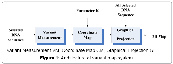
Figure 1: Architecture of variant map system.

Under this architecture, the component of Variant Measurement VM processes a selected DNA sequence with N elements as an input. Multiple segments can be partitioned into multiple segments and each segment composed of a fixed number of n elements. The output of the VM is composed of four vectors of probability measurement. The four vectors and a given k value are input data for the component of Coordinate Map CM, the output of the CM is a pair of position values created from input parameters. The pair of positions is an input parameter for the component of Graphical Projection GP to determine a projected position to be a visual point. After all elements of selected DNA sequences processed, multiple segments are transformed as a set of pair values to generate relevant graphs to indicate their distribution properties on 2D maps respectively.

Core modules

The VM component: The VM component is composed of three modules: Probability Measurement, Histograms and Normalized Histograms shown in Figure 2. The output of the VM component provides its output as the input of the CM component. Main I/O measures of the VM component are in three groups (Input, Intermediate and Output):

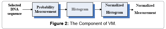
Figure 2: The Component of VM.

Input group:A selected DNA sequence

Intermediate output/input Group: Probability Measurement: Four sets of probability measurements on {A,C,G,T} projection respectively

Histograms: Histograms for relevant probability measurements

Output group

Normalized histograms: Normalized histograms for relevant probability measurements

The VM component: Four sets of probability measurements

The preprocessed DNA data forms multiple segments in a selected DNA sequence. The number of elements in each segment determines the horizontal coordinates; superpose the same number of segments to generate a histogram. Corresponding four {A,C,G,T} projections, four normalized histograms are created from the VM component. The values of each set of probability measurements are between 0 and 1, and the sum of each set is equal to 1.

The CM component

The CM component is shown as Figure 3 and its I/O parameters are listed as follows.

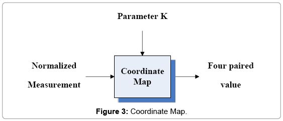
Figure 3: Coordinate Map.

Input group: Normalized Measurement: Four sets of probability measurements

K: An integer indicates the control parameter for mapping

Output group: Four paired values

This component takes probability measurements as input, using a control parameter k to generate relevant histogram and its normalized distribution. The output of this part is composed of four paired values in a given condition.

The GP component

The GP component is shown in Figure 4 and its I/O parameters are listed as follows.

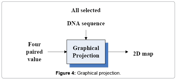
Figure 4: Graphical projection.

Input Group: All selected DNA sequence Four paired values

Output Group: Four 2D maps.

This part uses four paired values to repeat process rest segments in the selected DNA sequence. The output of this component provides four 2D maps as final output.

Detailed description

Section 2 provides system description on the Variant Map System, it is necessary to make further explanation for its further details in this section.

Parameter description

n an integer the number of elements in a segment, n>0

V a symbol selected from four DNA symbols, {A,G,T,C} = D, V ? D

K: An integer the control parameter for mapping

m_t: The t-th segments

: N j length in a j-th DNA sequencene

0 ≤ k ≤ N_j,0 < j < M, {(

: Four paired values, k>0, V ? D, {A, G, T, C} = D

Four sets of probability measurements

{H()} Four histograms for relevant probability measurements, V ? D, {A, G, T, C} = D

Four normalized histograms for relevant probability measurements, V ? D, {A, G, T, C} = D

Variant measurement

Multiple segments are partitioned by a fixed number of n elements for each segment from a selected DNA sequence length N, as the i-th packet. The number of each elements contained in a segment can be expressed as .

Counting this type of measures, a histogram can be created as H (Ti_v) satisfied the following condition:

Collecting all possible values, a histogram distribution can be established

Under this construction, a normalized histogram can be defined as

Coordinate map

Using this set of measurements, projective functions can be established to calculate a pair of values to analyze a DNA sequence into 2D map as follows:

Let

that will be a pair of values defined by following equations:

Then each pair of values locates a specific position on a 2D map for the selected DNA sequence.

Graphical projection

Each selected DNA sequence generates a specific position on a 2D map; it is essential to generate all selected sequence using graphical projection.

Each segment can get a specific position; the j-th position can be projected. Similar operations are repeated on other sequences and each sequence corresponding to a projective point on the 2D map. Consequently this part makes all processed measurements as their projective positions, and finally to generate four 2D maps for selected DNA sequences respectively.

Applying this system, coding and non-coding DNA sequences of genomes are selected from Multiple Species, and then eight groups of relevant variant maps are generated for each selected type of species.

Results of variant maps

It is always difficult to imagine map effects from control parameters in equations. A list of controlled effects will be illustrated in this section. Let readers easier understand different visual effects via different results of variant maps under various controlled parameters.

Sample results of variant maps on different parameters

Using coding and non-coding DNA sequences, under different conditions to illustrate their spatial distributions in a controllable environment. Group results under different k are shown in Figure 5.

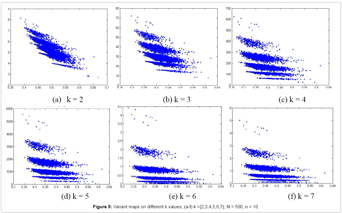
Figure 5: Variant maps on different k values; (a-f) k ={2,3,4,5,6,7}; N = 500, n = 10.

In Figure 5, six 2D maps are illustrated in the range of k = 2-7, N = 500, n = 10 for comparison, it seems that at k=4, map (e) provides a better distribution effect.

A set of results generated by various n is illustrated in Figure 6.

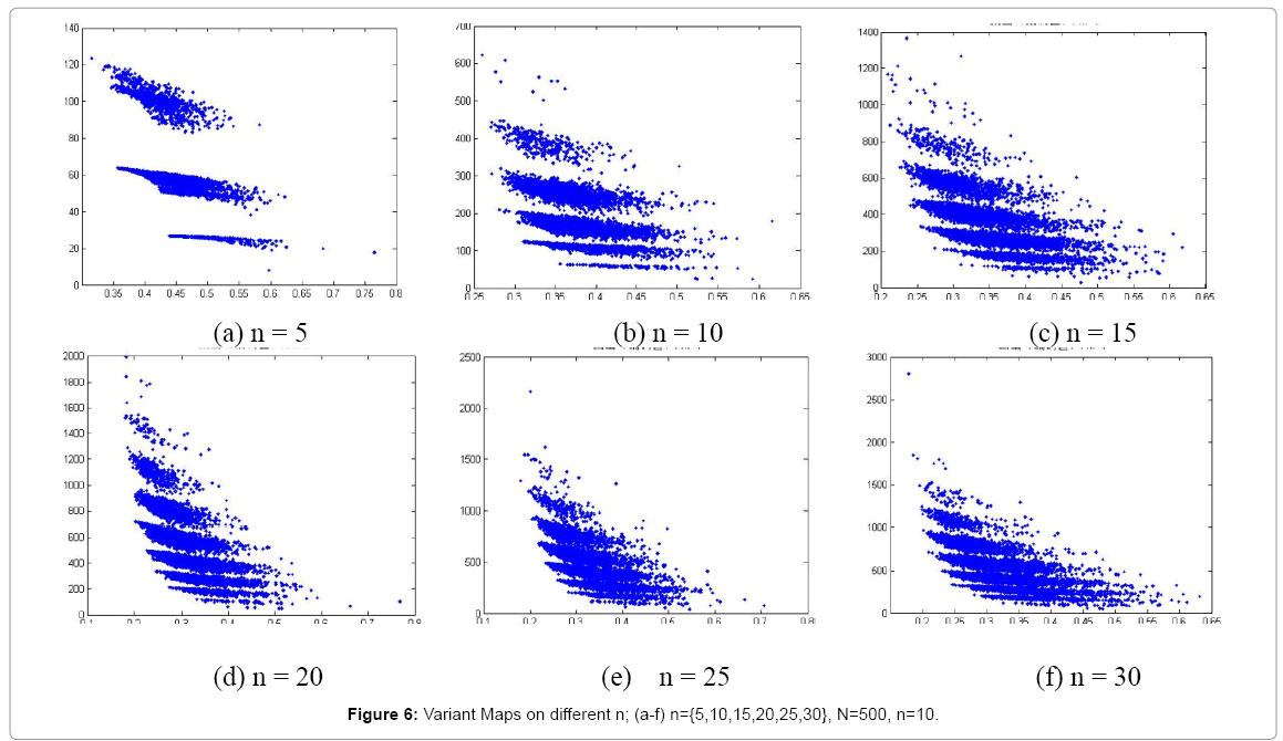
Figure 6: Variant Maps on different n; (a-f) n={5,10,15,20,25,30}, N=500, n=10.

In Figure 6, six 2D maps are selected in the range of k = 4, N=500, n = {5,10,15,20,25,30} conditions respectively. Map (b) may show a better distribution at n = 10.

In Figure 7, different maps are illustrated under n = 5 and k in different values.

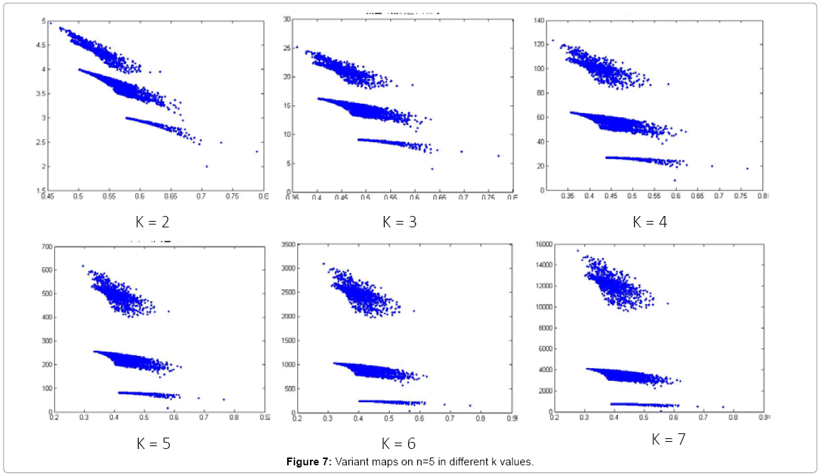
Figure 7: Variant maps on n=5 in different k values.

In Figure 7, six 2D maps are selected in condition on k = 2-7, N = 500, n = 5. Six maps do not have significant difference. By the reason, we select n=10 in further processes.

Variant maps on multiple species

Four species of DNA data sources are selected from worldwide public gene banks: Salmonella, Caenorhabditis Elegans, Oryza and Pan troglodytes.

A list of results will be shown in Figures 8-12 under different DNA data sequences and different control conditions.

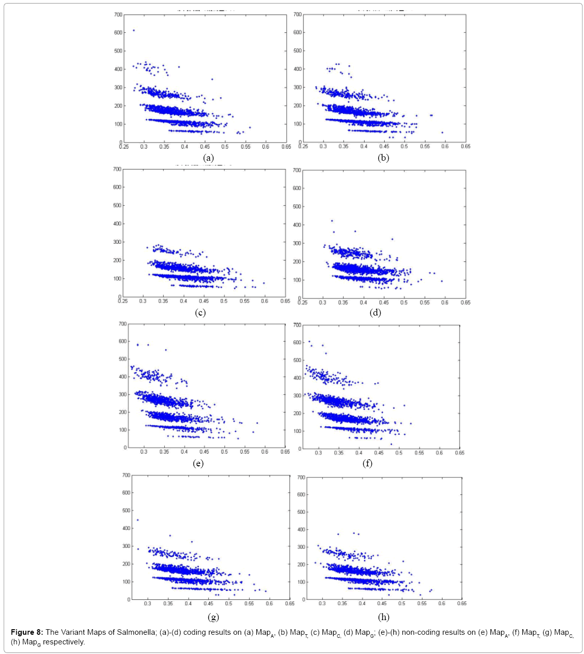
Figure 8: The Variant Maps of Salmonella; (a)-(d) coding results on (a) Map_A, (b) Map_T, (c) Map_C, (d) Map_G; (e)-(h) non-coding results on (e) Map_A, (f) Map_T, (g) Map_C, (h) Map_G respectively.

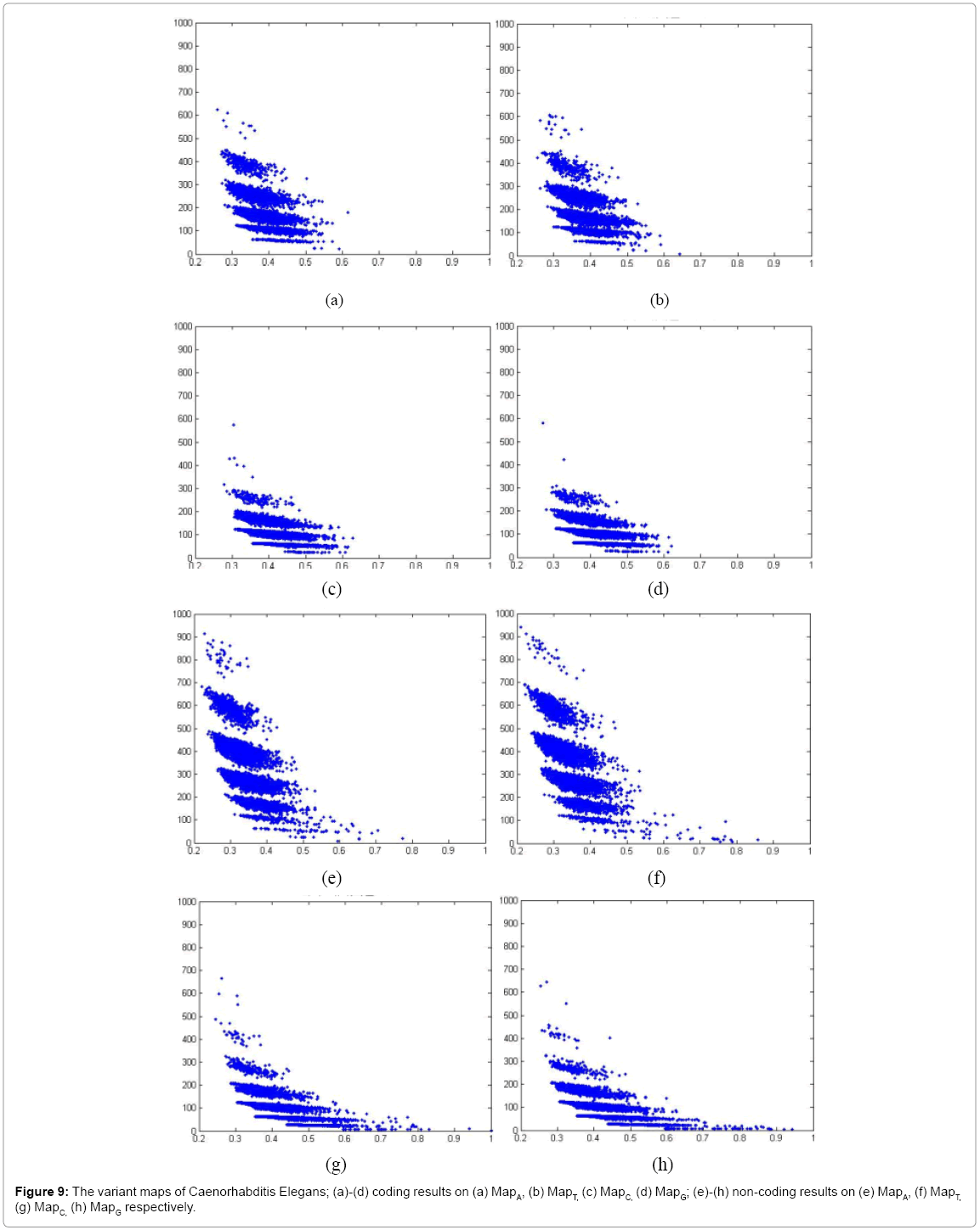
Figure 9: The variant maps of Caenorhabditis Elegans; (a)-(d) coding results on (a) Map_A, (b) Map_T, (c) Map_C, (d) Map_G; (e)-(h) non-coding results on (e) Map_A, (f) Map_T, (g) Map_C, (h) Map_G respectively.

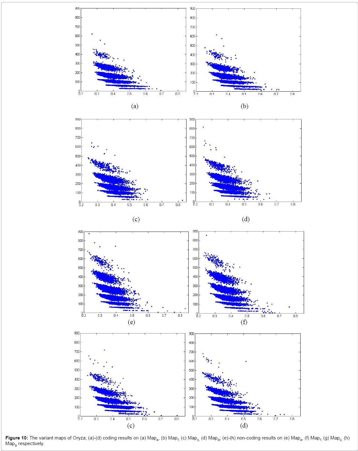
Figure 10: The variant maps of Oryza; (a)-(d) coding results on (a) Map_A, (b) Map_T, (c) Map_C, (d) Map_G; (e)-(h) non-coding results on (e) Map_A, (f) Map_T, (g) Map_C, (h) Map_G respectively.

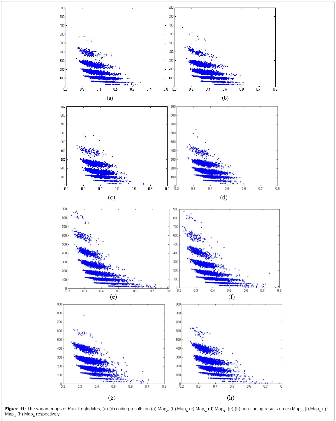
Figure 11: The variant maps of Pan Troglodytes; (a)-(d) coding results on (a) Map_A, (b) Map_T, (c) Map_C, (d) Map_G; (e)-(h) non-coding results on (e) Map_A, (f) Map_T, (g) Map_C, (h) Map_G respectively.

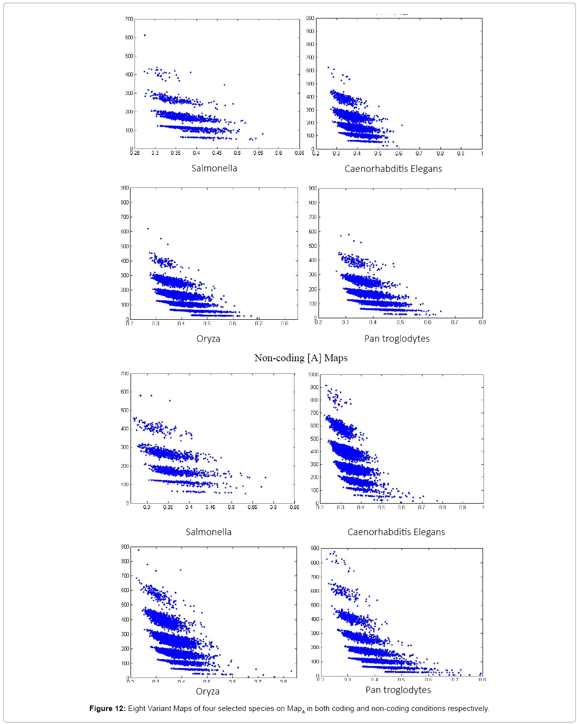
Figure 12: Eight Variant Maps of four selected species on Map_A in both coding and non-coding conditions respectively.

In Figure 8, eight variant maps of Salmonella are listed under the condition k=4, n=10, N=500. In which maps (a)–(d) are shown the results of coding DNA on MapA, MapT, MapC, MapG respectively. Maps (e)-(h) are shown the results of non-coding DNA on MapA, MapT, MapC, MapG respectively.

In Figure 9, eight variant maps of Caenorhabditis Elegans are listed under the condition k=4, n=10, N=500. In which maps (a)-(d) are shown the results of coding DNA on MapA, MapT, MapC, MapG respectively. Maps (e)-(h) are shown the result of non-coding DNA on MapA, MapT, MapC, MapG respectively

In Figure 10, eight variant maps of Oryza are listed under the condition k=4, n=10, N=500. In which Maps (a)-(d) are shown the results of coding DNA on MapA, MapT, MapC, MapG respectively. Maps (e)-(h) are shown the result of non-coding DNA on MapA, MapT, MapC, MapG respectively.

In Figure 11, eight variant maps of Pan troglodytes are listed under the condition k=4, n=10, N=500. In which Maps (a)-(d) are shown the results of coding DNA on MapA, MapT, MapC, MapG respectively. Maps (e)-(h) are shown the result of non-coding DNA on MapA, MapT, MapC, MapG respectively.

In Figure 12, eight variant maps are selected to show four variant maps of the four selected species on both coding and non-coding conditions especially on MapA selected under the condition k=4, n=10, N=500 respectively. Maps (a)-(d) are shown in coding cases and Maps (e)-(h) are shown in non-coding cases respectively.

In relation to 2D maps under different control parameters, 2D maps represent obviously different. At the region of n=10 and k=2-7, different distributions can be observed, k=4 maps may provide better separation effects shown in Figure 5.

It is interesting to observe different maps when parameter n changed. A larger n value makes a tighter distribution and larger n value takes clusters more separations on maps. Both n=5 and 10 maps may provide significant separation effects shown in Figure 6.

Six 2D maps are selected in the range of k=2-7, N=500, n=5 for comparison, they do not have significant differences shown in Figure 7. This indicates that smaller lengths of segment may not be good to illustrate the characteristics of the distribution.

Systematic illustrations are listed in Figures 9-11. Each Figure contains eight maps in which four of them are coding maps and another four maps are non-coding ones. On all listed maps, we can see obvious visual pairs of symmetric relationships on A-T & G-C in both coding and non-coding maps. In general, a stronger similar distribution among G-C can be easier observed. We can observe that Caenorhabditis Elegans, Oryza and Pan Troglodytes maps provide much better separation effects than Salmonella. The regions of distributions on noncoding maps are shown in much larger than relevant distributions of coding maps.

There are significant differences between coding and non-coding maps on Caenorhabditis Elegans, Oryza and Pan Troglodytes as distinct species, and their distributions of non-coding maps are with more substantial distinctions than coding maps.

Non-coding maps of four species as shown in Figure 12, Pan Troglodytes maps are shown very richer distributions, Caenorhabditis Elegans, Oryza maps are followed with richer effects, and Salmonella has simpler effects. From the genetic viewpoint, the Pan troglodytes belongs to higher level of animals, this specie has more similar to human genes to a higher degree, Caenorhabditis Elegans and Oryza are also higher creatures, but Salmonella are belong to much lower rank than others.

In a convenient comparison, Pan troglodytes’ maps show a richer distribution than other three. This set of results illustrates directly visual comparisons with significant differences between coding and non-coding DNA maps on different species in hierarchical organisms.

This paper proposes the variant map system to generate variant maps for four selected species. Using their selected DNA sequences respectively, this system uses variant measures, coordinate map and normalized histogram, to transform selected DNA sequences into significant different maps and each DNA sequence generates four projective maps on {A, T, G, C} respectively.

Using this type of multiple map schemes, it is convenient for Multiple Species to make relevant processing and comparison. Each selected DNA sequence can be distinguished by either coding or noncoding sequences. Their variant maps can be generated to illustrate their visual features to distinguish coding/non-coding cases. All listed species are contained very richer significant characteristics in their variant maps. This system can provide further usages to handle further R&D activities in coding and non-coding DNA/RNA sequences.

Thanks to the school of software engineering Yunnan University and the key laboratory of Yunnan software engineering for financial supports to this project.