Research Article - (2014) Volume 2, Issue 1
Keywords: Weather forecast; Statistical models
Despite advances in computing and satellite technologies and improvements in various atmospheric models scientists use to predict weather [1], there are still significant uncertainties in weather forecasts. Almost everyone has his or her own anecdotal experiences about the unreliability of weather forecasts. Some past studies have focused on the accuracies of forecasting severe weather conditions, such as tropical cyclones [2,3], but there have been fewer studies focused on quantifying the uncertainties of general every day weather forecasts, or comparing forecast accuracies across different geographical regions within the United States [4-6].
In this study, we make use of the historical forecast data from the National Oceanic and Atmospheric Administration’s see [7] National Weather Service Digital Library website see [8] to perform statistical analysis on the forecast accuracies of the most commonly watched weather forecasts: temperature, probability of precipitation, quantitative precipitation and wind speed. To compare geographical variations in forecast accuracies, we selected 60 geographical locations almost evenly spaced throughout the continental United States in terms of latitude and longitude1.
The main goal of this study is to focus on answering questions such as:
1. Statistically, do temperature forecasts do a better job than simply using the previous day’s number? Or, in other words, are the uncertainties of forecasts smaller than normal daily fluctuations?
2. When the forecast predicts a coming heat wave or calls for heavy rain, do they get it right, on the average, or do they over-or underpredict their target statistically speaking? What are the standard deviations of observed vs. predicted?
3. When the forecast calls for a 50% chance of precipitation, does it simply mean that they are not really sure whether it’s going to rain, or the weather model actually calculates a 50% probability? Does 50% chance of precipitation in Buffalo, NY mean the same thing as in Los Angeles, CA?
4. Among the weather variables, wind speeds are probably the most difficult to predict. But how uncertain are wind speed forecasts? Do the forecasters generally over or under forecast wind speeds?
5. Are there variations in weather forecast accuracies across different parts of the continental United States? Is it harder to predict rain or large change in temperature in the Great Lakes areas as compare to the Coastal Northeast?
Even though some of our analysis will be focusing on the occurrences of heat waves of over 10 degree temperature change or heavy precipitation of more than half an inch, the focus of our studies can still be characterized as high probability weather events. This is in contrast to studies of rare weather events such as tornados that could cause multi-billion dollar damages, or a flood with a 100-year recurrence interval. In principle one can also use the weather forecast database from the NWS Digital Library to study rare weather events. But since rare weather events happen at very low frequency, using general every day forecast database is less efficient.
Secondly, accessing forecast accuracies for rare weather events can be intrinsically difficult as the science for modeling these rare events continues to improve over the years. It is hard to measure the accuracy of a continuously improving forecast model for a rare weather event that happens once every hundred years.
For this study, we will use mean and standard deviation based statistical measures as opposed to composite scores for ranking purposes. We will give estimates for the sampling errors2 of the mean and standard deviation whenever appropriate. For example, for comparison purposes we will list the average daytime maximum temperature for different geographical locations, as well as their overall variations as measured by the standard deviations. For both of these measures, we will not list their sampling errors as the number of measurements is sufficiently large for this study. We will, however, give estimates of sampling errors for comparisons that have limited number of data points, e.g, The average forecast error for quantitative precipitation greater than 1.0 inches for Los Angeles, CA.
In the next section, we will give a brief description of the structure and type of weather data that was used in this study, and the software that we use to decode and access the database. We follow that with sections that discuss the main results for temperatures, precipitation, and wind speeds. Finally, we offer some ideas for future work and some potential practical applications of our findings.
Weather data are typically stored in binary format known as the GRIB [Gridded Binary] format. This format is used by most of the world to store weather related data. It contains standardized header information that can be read by a variety of software packages3. The web site we used to download historical weather forecasts are maintained by the National Environmental Satellite, Data, and Information Services’ National Climate Data Center see [9] under the US Department of Commerce. The data set is extremely comprehensive and covers time periods from 2004 to present. It is freely available to anyone who is interested in studying weather data, but one generally needs a very high speed internet connection to be able to download the data in any reasonable amount of time.
The files are identified primarily by their WMO [World Meteorological Organization] header codes. For example, files that start with ‘YG’ will contain daytime maximum temperature, and ‘YD’ files will have data for probability of precipitation. Lists of the some of these WMO codes are listed in Table 1.
| WMO Code | Description | WMO Code | Description |
|---|---|---|---|
| YB | Wind Direction (surface) | YI | Quantitative Precipitation |
| YC | Wind Speed (surface) | YR | Relative Humidity |
| YD | Probability of Precipitation | YS | Snowfall Amount |
| YE | Surface Temperature | YT | Apparent Temperature |
| YG | Daytime Max Temperature | YW | Wind Gust Speed |
| YH | Nightime Min Temperature | LE | Probability of Tornado |
Table 1: WMO Code Descriptions.
In this study, we will analyze data from the time period of January 2009 to June 2013. Since each day is one file, for each WMO code, there are approximately 1,600 files to download. The file sizes vary depending on the type of weather data, but they range between 50 MB to 200 MB each4. The total amount of data eventually downloaded ads up to approximately 2TB5. To read the binary formatted GRIB data, we used the Degrib see [10,11] software package. Degrib works by probing the data for a particular geographical location using a pair of latitude and longitude for the location. In this study, we chose 60 geographical locations roughly evenly spaced throughout the continental United States6. Since GRIB data are structured around the latitude and longitude grid [using bi-linear interpolations between points7], ideally one should select a grid with fixed spacing between grid points, but for this study, we will use mostly metropolitan area for the purposes of easy name recognitions.
For post processing of the GRIB data, we extract the relevant weather measure for each geographical location for the entire 2009- 2013 time period and put them all in one data file. For example, we would extract daytime maximum temperature data for Los Angeles, CA from the approximately 1,600 “YG” files into one single file. This makes processing all 60 geographical locations easier and faster as one does not need to go through a large GRIB file for each geographical location, as well as saving time from having to access large number of files.
In this part, the first sets of questions we will attempt to answer are: What is magnitude of the overall error in daytime maximum temperature forecasts? Are there statistically significant geographical differences? If so, would those differences correlate to the location’s overall volatilities of temperature changes?
For 6-day forecast results, Table 2 ranks overall forecast errors as the standard deviation of actual minus forecast  . This analysis shows that the forecast errors in most cases are similar in magnitude to the day-to-day change in actual temperature. At first glance, this might seem to indicate that the 6-day forecasts do not seem to provide much value in terms of forecasting, as someone randomly make up some numbers would give you the same standard errors as day-to-day fluctuations. What we need to keep in mind here, however, is that the results listed here are simply overall averages. They do not imply that the forecasters are completely incapable of forecasting anything 6 days ahead. It simply means that the forecast errors are fairly large, on the average. In other words, it could mean that forecasters can be off by the same error, for both normal days and days that have large changes in temperature.
| Location |  |
 |
 |
|
 |
Location | |
|
|
|
|
| Great Falls, MT | 9.99 | -0.01 | 0.22 | 8.64 | 0.87 | Idaho Falls, ID | 6.22 | -0.05 | 0.15 | 5.8 | 0.93 |
| Denver, CO | 10.35 | 0.01 | 0.2 | 8.1 | 0.78 | Pasadena, CA | 6 | -0.45 | 0.14 | 5.75 | 0.96 |
| Amarillo, TX | 10.41 | 0.51 | 0.2 | 7.95 | 0.76 | New York, NY | 7.22 | 0.78 | 0.14 | 5.74 | 0.79 |
| Bismarck, ND | 9.18 | 0.16 | 0.19 | 7.7 | 0.84 | Reno, NV | 6.65 | -0.1 | 0.14 | 5.71 | 0.86 |
| Wichita, KS | 9.49 | 0.73 | 0.19 | 7.6 | 0.8 | Boise, ID | 6.17 | 0.35 | 0.14 | 5.61 | 0.91 |
| Riverton, WY | 8 | -0.63 | 0.18 | 7.29 | 0.91 | Mammoth, CA | 6.27 | -0.43 | 0.14 | 5.58 | 0.89 |
| Sioux Falls, SD | 8.94 | 0.38 | 0.18 | 7.21 | 0.81 | Atlanta, GA | 5.98 | -0.14 | 0.14 | 5.48 | 0.92 |
| St. Louis, MO | 9.13 | 0.7 | 0.18 | 7.14 | 0.78 | Santa Fe, NM | 6 | 0.68 | 0.14 | 5.46 | 0.91 |
| Boston, MA | 8.32 | 0.22 | 0.17 | 6.71 | 0.81 | Charlotte, NC | 6.84 | 0.43 | 0.14 | 5.41 | 0.79 |
| Burlington, VT | 8.37 | 0 | 0.17 | 6.7 | 0.8 | San Luis Obispo, CA | 5.41 | 0.14 | 0.13 | 5.34 | 0.99 |
| John Day, OR | 6.89 | -1.28 | 0.17 | 6.66 | 0.97 | Spokane, WA | 6.03 | -0.13 | 0.13 | 5.34 | 0.89 |
| Dallas, TX | 8.2 | -0.15 | 0.17 | 6.63 | 0.81 | South Lake Tahoe, CA | 6.15 | 0.15 | 0.13 | 5.32 | 0.87 |
| Augusta, ME | 7.61 | 0.08 | 0.16 | 6.54 | 0.86 | Flagstaff, AZ | 5.77 | -0.44 | 0.13 | 5.24 | 0.91 |
| Chicago, IL | 8.51 | 0.43 | 0.16 | 6.51 | 0.76 | Wilmington, NC | 6.73 | -0.16 | 0.13 | 5.23 | 0.78 |
| Duluth, MN | 7.86 | 0.54 | 0.16 | 6.46 | 0.82 | Roseburg, OR | 5.64 | -0.32 | 0.13 | 5.23 | 0.93 |
| Charleston, WV | 8.4 | 0.8 | 0.16 | 6.43 | 0.77 | Las Cruces, NM | 5.67 | -0.73 | 0.13 | 5.01 | 0.88 |
| Little Rock, AR | 7.84 | 0.07 | 0.16 | 6.38 | 0.81 | Palm Springs, CA | 5.1 | -0.21 | 0.13 | 4.98 | 0.98 |
| Warm Springs, VA | 7.87 | 0.68 | 0.16 | 6.26 | 0.79 | Portland, OR | 5.22 | -0.06 | 0.12 | 4.97 | 0.95 |
| Milwaukee, WI | 8.31 | 0.22 | 0.16 | 6.24 | 0.75 | Los Angeles, CA | 5.02 | -0.12 | 0.12 | 4.96 | 0.99 |
| Cleveland, OH | 8.25 | 0.69 | 0.15 | 6.15 | 0.75 | Phoenix, AZ | 5.31 | -0.12 | 0.12 | 4.93 | 0.93 |
| Cincinnati, OH | 8.08 | 0.27 | 0.15 | 6.14 | 0.76 | Houston, TX | 5.98 | 0.53 | 0.12 | 4.82 | 0.81 |
| Portland, ME | 7.22 | 0.24 | 0.15 | 6.12 | 0.85 | Jacksonville, FL | 5.83 | -0.01 | 0.12 | 4.73 | 0.81 |
| Nashville, TN | 8 | -0.12 | 0.15 | 6.11 | 0.76 | Seattle, WA | 4.63 | 0.18 | 0.12 | 4.68 | 1.01 |
| Baltimore, MD | 7.74 | 0.23 | 0.15 | 6.04 | 0.78 | Las Vegas, NV | 5.09 | -0.24 | 0.12 | 4.68 | 0.92 |
| Albany, NY | 7.56 | 0.37 | 0.15 | 6.01 | 0.8 | Merced, CA | 4.87 | -0.1 | 0.12 | 4.64 | 0.95 |
| Buffalo, NY | 8.21 | -0.45 | 0.15 | 6 | 0.73 | San Jose, CA | 4.85 | 0.06 | 0.12 | 4.6 | 0.95 |
| Battle Mountain, NV | 7 | -0.29 | 0.15 | 6 | 0.86 | Santa Monica, CA | 4.41 | -0.13 | 0.11 | 4.51 | 1.02 |
| Flint. MI | 7.58 | 0.49 | 0.15 | 5.95 | 0.78 | Mobile, AL | 4.93 | -0.28 | 0.11 | 4.43 | 0.9 |
| Redding, CA | 6.11 | 0.03 | 0.15 | 5.94 | 0.97 | San Francisco, CA | 4.15 | -0.03 | 0.1 | 4.1 | 0.99 |
| Salt Lake City, UT | 6.84 | -0.21 | 0.15 | 5.92 | 0.87 | Miami, FL | 3.65 | -0.5 | 0.08 | 3.31 | 0.91 |
Note: is the standard deviation of actual day-to-day change, is the mean of actual minus 6-day forecast, is the estimated sampling error of the mean, and is the standard deviation of actual minus forecast
Table 2: Daytime high temperature 6-day forecast vs actual, ranked by the standard deviation of forecast errors.
In Table 2, we also list the ratios of the forecast errors to the standard deviations of day-to-day changes. We see that there are fairly large variations in terms of this ratio for the geographical locations listed8. The highest being that of Santa Monica, CA and many locations in California, and the lowest are generally those that have fairly large day-to-day changes in temperatures. This could mean that predicting daytime maximum temperatures in many parts of California (especially those close to the coast) could be just random guesses for most days as the day-to-day fluctuations are relatively small, and the 6-day horizon is simply too long to make precise forecasts. On the other hand, large day-to-day temperatures changes for many areas could most likely be due to tangible weather events, and forecasters might have an easier job in those cases.
The mean of actual minus forecast listed in Table 2 are mostly zeros within the sampling errors, indicating that there are no apparent biases, either high or low, for the majority of the locations considered. But some areas do show statistically consistent biases in actual minus forecast. For example, forecasters tend to over-forecast daytime high temperature by an average of about 0.8°F for New York City, and under-forecast by 0.7°F in Las Cruces, NM.
Not surprising, 3-day forecasts are more accurate than 6-day forecasts, as shown in Table 3. The average errors are still fairly large, however, e.g., at 5.2°F for Wichita, KS, and 4.5°F for Dallas, TX. The improvements are relatively modest for many West Coast locations in terms of absolute temperature, but the percent changes relative to day-to-day temperature fluctuations are similar overall [about 40% improvements].
| Location | |
 |
 |
 |
 |
Location | |
|
|
|
|
| Great Falls, MT | 10.14 | 0 | 0.14 | 5.47 | 0.54 | Charlotte, NC | 6.82 | 0.01 | 0.09 | 3.73 | 0.55 |
| Wichita, KS | 9.46 | 0.58 | 0.13 | 5.16 | 0.54 | Mammoth, CA | 6.27 | -0.09 | 0.09 | 3.72 | 0.59 |
| Amarillo, TX | 10.33 | 0.44 | 0.13 | 5.14 | 0.5 | Pasadena, CA | 5.98 | -0.24 | 0.09 | 3.7 | 0.62 |
| Bismarck, ND | 9.09 | 0.22 | 0.13 | 5.09 | 0.56 | Battle Mountain, NV | 7.04 | -0.06 | 0.09 | 3.65 | 0.52 |
| Denver, CO | 10.35 | 0.1 | 0.13 | 5.01 | 0.48 | Salt Lake City, UT | 6.82 | 0.02 | 0.09 | 3.59 | 0.53 |
| St. Louis, MO | 9.24 | 0.7 | 0.13 | 5 | 0.54 | San Luis Obispo, CA | 5.34 | 0.08 | 0.09 | 3.58 | 0.67 |
| Burlington, VT | 8.43 | -0.27 | 0.12 | 4.81 | 0.57 | Idaho Falls, ID | 6.23 | 0.06 | 0.09 | 3.56 | 0.57 |
| Boston, MA | 8.29 | -0.12 | 0.12 | 4.79 | 0.58 | Spokane, WA | 6.05 | -0.13 | 0.09 | 3.56 | 0.59 |
| Chicago, IL | 8.66 | 0.45 | 0.12 | 4.67 | 0.54 | Roseburg, OR | 5.59 | -0.11 | 0.09 | 3.52 | 0.63 |
| Little Rock, AR | 7.88 | -0.04 | 0.12 | 4.65 | 0.59 | Reno, NV | 6.62 | 0.14 | 0.09 | 3.5 | 0.53 |
| Sioux Falls, SD | 8.89 | 0.57 | 0.12 | 4.6 | 0.52 | Redding, CA | 6.06 | 0.1 | 0.09 | 3.5 | 0.58 |
| Augusta, ME | 7.59 | -0.67 | 0.11 | 4.56 | 0.6 | Phoenix, AZ | 5.33 | -0.15 | 0.09 | 3.49 | 0.65 |
| Dallas, TX | 8.31 | -0.11 | 0.11 | 4.5 | 0.54 | Boise, ID | 6.16 | 0.27 | 0.09 | 3.45 | 0.56 |
| Charleston, WV | 8.49 | 0.75 | 0.11 | 4.49 | 0.53 | Flagstaff, AZ | 5.74 | -0.01 | 0.08 | 3.38 | 0.59 |
| Riverton, WY | 8.02 | 0 | 0.11 | 4.46 | 0.56 | Santa Fe, NM | 6.03 | 0.53 | 0.08 | 3.38 | 0.56 |
| Warm Springs, VA | 7.91 | 0.15 | 0.11 | 4.45 | 0.56 | Los Angeles, CA | 5 | -0.05 | 0.08 | 3.38 | 0.68 |
| John Day, OR | 6.89 | -0.99 | 0.11 | 4.37 | 0.63 | Palm Springs, CA | 5.08 | -0.05 | 0.08 | 3.37 | 0.66 |
| Duluth, MN | 7.8 | 0.63 | 0.11 | 4.36 | 0.56 | Jacksonville, FL | 5.91 | -0.18 | 0.08 | 3.33 | 0.56 |
| Nashville, TN | 8.09 | -0.3 | 0.11 | 4.36 | 0.54 | San Francisco, CA | 4.13 | -0.02 | 0.08 | 3.31 | 0.8 |
| Milwaukee, WI | 8.4 | 0.37 | 0.11 | 4.35 | 0.52 | Houston, TX | 6.04 | 0.33 | 0.08 | 3.29 | 0.54 |
| Buffalo, NY | 8.24 | -0.28 | 0.11 | 4.34 | 0.53 | Santa Monica, CA | 4.4 | -0.09 | 0.08 | 3.27 | 0.74 |
| Baltimore, MD | 7.61 | 0.14 | 0.11 | 4.32 | 0.57 | Las Cruces, NM | 5.67 | -0.22 | 0.08 | 3.23 | 0.57 |
| New York, NY | 7.15 | 0.64 | 0.11 | 4.31 | 0.6 | South Lake Tahoe, CA | 6.17 | 0.3 | 0.08 | 3.23 | 0.52 |
| Cincinnati, OH | 8.16 | 0.19 | 0.11 | 4.31 | 0.53 | Merced, CA | 4.81 | -0.03 | 0.08 | 3.11 | 0.65 |
| Portland, ME | 7.19 | -0.45 | 0.11 | 4.28 | 0.59 | Mobile, AL | 4.99 | -0.51 | 0.08 | 3.08 | 0.62 |
| Albany, NY | 7.57 | -0.44 | 0.11 | 4.26 | 0.56 | Portland, OR | 5.17 | 0.01 | 0.08 | 3.06 | 0.59 |
| Cleveland, OH | 8.31 | 0.46 | 0.11 | 4.24 | 0.51 | Seattle, WA | 4.62 | 0.1 | 0.08 | 3.02 | 0.65 |
| Flint. MI | 7.69 | 0.55 | 0.1 | 4.1 | 0.53 | San Jose, CA | 4.83 | -0.03 | 0.07 | 2.91 | 0.6 |
| Atlanta, GA | 5.98 | -0.31 | 0.1 | 3.87 | 0.65 | Las Vegas, NV | 5.09 | -0.09 | 0.07 | 2.81 | 0.55 |
| Wilmington, NC | 6.74 | -0.32 | 0.1 | 3.82 | 0.57 | Miami, FL | 3.68 | -0.32 | 0.06 | 2.56 | 0.7 |
Table 3: Daytime high temperature 3-day forecast vs actual, ranked by the standard deviations of forecast errors.
Having looked at overall average errors, we examine next how well forecasters are able to forecast large swings in daytime high temperatures. We first look at days when the actual temperature at the forecast date differs by a large amount from that of the previous day9. In other words, for 3-day forecasts, we will look at T[3]- f[3] given that Ta[3]-Ta[2] ≥ C, or Ta[3]-Ta[2]≤ - C. Here the subscript a means actual, f means forecasted, and C could be a large cutoff constant, say 10°F. Table 4 shows the results as ranked by the mean of the actual minus forecasted. Here the results clearly indicate that for most of the areas, the forecasters significantly under-forecast the daytime high if the temperature experienced a surge of at least 10°F from the previous day. For example, the forecasters under-predicted daytime high on the average by 4.2°F for New York City. There are strong variations among the 60 geographical regions considered, but with no apparent correlations to the variations shown in Table 3. For some locations, the averages of the forecast errors are similar in magnitude to the standard deviations of the forecast errors.
| Location | |
|
|
Location | |
|
|
| San Francisco, CA | 6.69 | 1.65 | 7.21 | Wilmington, NC | 2.69 | 0.45 | 4.23 |
| Charleston, WV | 4.45 | 0.38 | 4.41 | Portland, OR | 2.67 | 0.47 | 3.08 |
| San Luis Obispo, CA | 4.21 | 0.49 | 3.11 | Spokane, WA | 2.65 | 0.53 | 3.99 |
| St. Louis, MO | 4.2 | 0.4 | 4.58 | Augusta, ME | 2.64 | 0.43 | 4.92 |
| New York, NY | 4.16 | 0.43 | 4.72 | Denver, CO | 2.51 | 0.27 | 3.78 |
| Los Angeles, CA | 4.15 | 0.54 | 3.03 | Seattle, WA | 2.5 | 0.93 | 3.93 |
| Wichita, KS | 4.13 | 0.41 | 5.16 | Mammoth, CA | 2.47 | 0.64 | 4.88 |
| Milwaukee, WI | 4.07 | 0.44 | 5.07 | Albany, NY | 2.45 | 0.38 | 4.25 |
| Baltimore, MD | 3.86 | 0.46 | 5.01 | Flagstaff, AZ | 2.36 | 0.41 | 3.17 |
| Flint. MI | 3.86 | 0.47 | 4.7 | Salt Lake City, UT | 2.3 | 0.49 | 4.39 |
| Cleveland, OH | 3.68 | 0.33 | 3.82 | Dallas, TX | 2.27 | 0.38 | 3.98 |
| Duluth, MN | 3.59 | 0.39 | 4.34 | Idaho Falls, ID | 2.2 | 0.66 | 4.68 |
| Sioux Falls, SD | 3.47 | 0.34 | 4.28 | Houston, TX | 2.19 | 0.45 | 3.27 |
| Santa Monica, CA | 3.43 | 0.63 | 2.75 | Las Cruces, NM | 2.17 | 0.59 | 3.66 |
| Boston, MA | 3.41 | 0.41 | 5.09 | Jacksonville, FL | 2.14 | 0.49 | 3.76 |
| Cincinnati, OH | 3.4 | 0.44 | 4.83 | Burlington, VT | 2.09 | 0.35 | 4.32 |
| Warm Springs, VA | 3.38 | 0.32 | 3.58 | Redding, CA | 2.09 | 0.42 | 3.47 |
| San Jose, CA | 3.36 | 0.75 | 3.95 | Roseburg, OR | 2.03 | 0.46 | 3.25 |
| Merced, CA | 3.35 | 1.36 | 5.92 | South Lake Tahoe, CA | 1.91 | 0.6 | 4.54 |
| Portland, ME | 3.32 | 0.43 | 4.55 | Great Falls, MT | 1.84 | 0.44 | 5.95 |
| Little Rock, AR | 3.07 | 0.43 | 4.67 | Riverton, WY | 1.8 | 0.47 | 5.37 |
| Chicago, IL | 2.98 | 0.45 | 5.19 | Reno, NV | 1.8 | 0.53 | 4.3 |
| Boise, ID | 2.95 | 0.64 | 4.53 | Atlanta, GA | 1.75 | 0.5 | 3.75 |
| Charlotte, NC | 2.93 | 0.4 | 3.79 | Battle Mountain, NV | 1.63 | 0.49 | 4.31 |
| Nashville, TN | 2.88 | 0.43 | 4.26 | John Day, OR | 1.5 | 0.39 | 3.79 |
| Buffalo, NY | 2.88 | 0.46 | 5.21 | Palm Springs, CA | 1.3 | 0.65 | 2.76 |
| Mobile, AL | 2.85 | 0.58 | 3.12 | Las Vegas, NV | 1.11 | 0.8 | 3.58 |
| Bismarck, ND | 2.84 | 0.42 | 5.4 | Phoenix, AZ | 1.1 | 0.85 | 4.06 |
| Amarillo, TX | 2.84 | 0.35 | 4.78 | Santa Fe, NM | 0.85 | 0.49 | 3.43 |
| Pasadena, CA | 2.83 | 0.42 | 3.05 | Miami, FL | 0.56 | 1.5 | 4.5 |
Table 4: Daytime maximum temperature 3-day forecast vs actual when 10°F ≤ T(3)-Ta(2) ≤ 20°F, as ranked by , the mean of actual minus 3-day forecasted.
In this section, we look at results of actual probabilities of precipitation vs. forecasted probabilities. Here the actual probability is calculated by taking the total number of days that forecasters predicted rain with a certain probability, and divide that by the actual number of days that actually experienced precipitation. For example, let’s say we want to assess what is the actual realized probability of 20% chance of rain. We first find the total number of days that the forecasters predicted a 20% chance of rain 3 days ahead. We then divide that by the total number of days that actually rained on the dates that the forecasters referenced to [in their 3-day forecasts].
Table 5 shows the actual probabilities10 of precipitation for both 20%-50% and 50%-70% chances of 3-day forecasted precipitation. The results are ranked by their actual probabilities for the 20%-50% chance forecasts11. The results in this table seem to indicate that actual probabilities of precipitation can be significantly lower than forecasted, especially for probabilities below 50%. Additionally, the geographical differences in actual realized probabilities can differ by as much as an order of magnitude. The variations in actual probabilities for the 50%- 70% range seem to be less than that for the 20%-50% range, but the differences are still significant. In other words, when the 3-day forecast calls for a chance of precipitation in the range of 20%-50%12, the actual chance of precipitation is much lower than the forecasts, on the average. For example, for San Jose, CA, the average actual probability is only 4.8%, significantly lower than the lower bound value of the forecasted, which is 20%. But the average actual probability goes up to 26% if the forecasted is between 50% to 70%. This is still much lower than the lower bound of the forecasted, but the difference here is somewhat smaller.
| Location |  |
 |
 |
 |
Location | |
|
|
|
| Flint. MI | 15.90% | 0.90% | 42.10% | 2.30% | Merced, CA | 7.40% | 1.30% | 23.20% | 3.10% |
| Milwaukee, WI | 15.60% | 1.00% | 44.10% | 2.60% | Seattle, WA | 7.30% | 0.70% | 23.80% | 1.50% |
| Baltimore, MD | 14.90% | 0.90% | 45.30% | 2.60% | Pasadena, CA | 7.30% | 1.40% | 44.30% | 5.00% |
| Boston, MA | 14.40% | 0.90% | 43.40% | 2.30% | Wichita, KS | 7.20% | 0.80% | 33.30% | 3.50% |
| Buffalo, NY | 13.40% | 0.80% | 37.80% | 1.80% | Cleveland, OH | 7.00% | 0.60% | 33.10% | 1.60% |
| Chicago, IL | 13.30% | 0.90% | 45.30% | 2.70% | Santa Monica, CA | 6.90% | 1.40% | 43.60% | 5.00% |
| Cincinnati, OH | 12.10% | 0.80% | 41.60% | 2.20% | Albany, NY | 6.60% | 0.60% | 30.40% | 1.90% |
| Sioux Falls, SD | 11.90% | 0.90% | 41.00% | 2.80% | Duluth, MN | 6.40% | 0.60% | 31.60% | 2.50% |
| South Lake Tahoe, CA | 11.60% | 1.10% | 37.20% | 3.00% | Salt Lake City, UT | 6.40% | 0.70% | 30.00% | 2.40% |
| Wilmington, NC | 10.30% | 0.80% | 42.30% | 3.10% | Redding, CA | 6.30% | 0.90% | 35.00% | 2.80% |
| New York, NY | 10.10% | 0.70% | 36.60% | 2.00% | St. Louis, MO | 5.90% | 0.70% | 23.90% | 2.20% |
| Great Falls, MT | 9.50% | 0.80% | 38.90% | 2.90% | Denver, CO | 5.70% | 0.70% | 43.70% | 5.20% |
| Charleston, WV | 9.40% | 0.70% | 28.10% | 1.70% | Battle Mountain, NV | 5.50% | 0.80% | 20.80% | 3.80% |
| Portland, OR | 9.30% | 0.80% | 31.70% | 1.80% | Mammoth, CA | 5.10% | 0.80% | 30.80% | 3.30% |
| Bismarck, ND | 9.00% | 0.80% | 43.70% | 3.40% | Nashville, TN | 4.90% | 0.60% | 25.50% | 2.00% |
| Charlotte, NC | 8.80% | 0.70% | 37.00% | 2.50% | Little Rock, AR | 4.80% | 0.60% | 27.00% | 2.30% |
| Roseburg, OR | 8.70% | 0.90% | 31.00% | 1.90% | San Jose, CA | 4.80% | 1.00% | 26.00% | 2.90% |
| Reno, NV | 8.70% | 1.00% | 25.90% | 3.40% | Palm Springs, CA | 4.30% | 1.40% | 11.80% | 6.50% |
| Los Angeles, CA | 8.70% | 1.60% | 48.00% | 5.30% | San Francisco, CA | 4.00% | 0.90% | 27.50% | 3.00% |
| Burlington, VT | 8.60% | 0.70% | 32.10% | 1.80% | Flagstaff, AZ | 3.20% | 0.60% | 28.90% | 3.10% |
| Dallas, TX | 8.00% | 0.90% | 35.80% | 3.70% | Phoenix, AZ | 3.20% | 0.90% | 28.60% | 8.10% |
| Riverton, WY | 8.00% | 0.90% | 41.50% | 4.20% | Mobile, AL | 3.20% | 0.50% | 23.10% | 2.20% |
| San Luis Obispo, CA | 8.00% | 1.40% | 31.90% | 3.60% | Jacksonville, FL | 2.10% | 0.40% | 12.90% | 1.90% |
| Augusta, ME | 7.90% | 0.70% | 36.50% | 2.10% | John Day, OR | 2.00% | 0.40% | 12.00% | 1.70% |
| Spokane, WA | 7.90% | 0.80% | 34.60% | 2.20% | Las Vegas, NV | 2.00% | 0.80% | 17.20% | 5.70% |
| Boise, ID | 7.80% | 0.80% | 25.40% | 3.20% | Idaho Falls, ID | 1.50% | 0.30% | 14.30% | 2.40% |
| Amarillo, TX | 7.70% | 1.00% | 34.40% | 7.10% | Houston, TX | 1.40% | 0.30% | 15.20% | 2.20% |
| Portland, ME | 7.60% | 0.70% | 39.00% | 2.20% | Las Cruces, NM | 1.00% | 0.50% | 16.70% | 12.40% |
| Warm Springs, VA | 7.50% | 0.60% | 29.60% | 2.10% | Miami, FL | 0.80% | 0.20% | 6.50% | 1.70% |
| Atlanta, GA | 7.50% | 0.70% | 40.80% | 2.80% | Santa Fe, NM | 0.60% | 0.30% | 6.30% | 5.20% |
Table 5: Actual probabilities of precipitation for two ranges of 3-day forecasts: (1) 20%-50%, and (2) 50%-70%. Here is the actual realized probability of precipitation, and is the sampling error of . The locations are ranked by their values.
For comparisons, actual probabilities corresponding to shorter horizon forecast is shown in Table 6. The results seem to indicate that realized probabilities are noticeably smaller for 1-day forecasts as compared to that of 3-day forecasts for same 50%-70% range of forecasted probabilities [with a higher dispersion of geographical variations]. In other words, 3-day forecasts seem to be more accurate than 1-day forecasts if the forecasted chance falls between 50%-70%.
| Location |  |
 |
Location | |
|
| Boston, MA | 27.60% | 2.10% | Warm Springs, VA | 11.70% | 1.40% |
| Cincinnati, OH | 25.90% | 2.00% | St. Louis, MO | 11.70% | 1.60% |
| Chicago, IL | 25.70% | 2.00% | Cleveland, OH | 11.50% | 1.20% |
| Sioux Falls, SD | 25.50% | 2.20% | Denver, CO | 11.30% | 2.10% |
| Buffalo, NY | 24.00% | 1.70% | Duluth, MN | 10.70% | 1.40% |
| Flint. MI | 22.20% | 1.70% | Salt Lake City, UT | 10.60% | 1.40% |
| Amarillo, TX | 21.70% | 3.70% | Little Rock, AR | 9.90% | 1.60% |
| Wilmington, NC | 21.60% | 2.20% | Redding, CA | 9.60% | 2.00% |
| Riverton, WY | 21.30% | 2.90% | Roseburg, OR | 9.40% | 1.40% |
| Milwaukee, WI | 20.70% | 2.00% | Palm Springs, CA | 9.40% | 4.30% |
| Great Falls, MT | 20.60% | 2.20% | Albany, NY | 9.20% | 1.30% |
| Baltimore, MD | 20.00% | 1.80% | Phoenix, AZ | 9.10% | 3.60% |
| Augusta, ME | 16.40% | 1.70% | Nashville, TN | 8.60% | 1.30% |
| Burlington, VT | 16.40% | 1.60% | Merced, CA | 8.60% | 2.30% |
| Bismarck, ND | 16.10% | 1.90% | Boise, ID | 7.90% | 1.50% |
| Atlanta, GA | 15.90% | 1.80% | Battle Mountain, NV | 7.70% | 1.80% |
| Portland, ME | 15.70% | 1.80% | San Luis Obispo, CA | 7.00% | 2.20% |
| Spokane, WA | 15.70% | 1.60% | San Francisco, CA | 7.00% | 1.70% |
| Charlotte, NC | 15.40% | 1.70% | Seattle, WA | 6.50% | 1.00% |
| Wichita, KS | 14.80% | 2.10% | Jacksonville, FL | 6.40% | 1.20% |
| Los Angeles, CA | 14.30% | 3.10% | Flagstaff, AZ | 5.90% | 1.40% |
| South Lake Tahoe, CA | 14.10% | 2.30% | Mobile, AL | 5.40% | 1.10% |
| Dallas, TX | 14.00% | 2.20% | Las Vegas, NV | 5.10% | 2.50% |
| Santa Monica, CA | 13.90% | 3.20% | John Day, OR | 4.30% | 0.90% |
| Pasadena, CA | 13.40% | 3.10% | Santa Fe, NM | 3.80% | 1.70% |
| Mammoth, CA | 13.40% | 2.50% | Houston, TX | 3.30% | 1.10% |
| New York, NY | 12.60% | 1.60% | Idaho Falls, ID | 2.50% | 0.90% |
| Reno, NV | 12.40% | 2.30% | Las Cruces, NM | 2.30% | 2.00% |
| Portland, OR | 11.90% | 1.40% | Miami, FL | 2.20% | 0.80% |
| harleston, WV | 11.80% | 1.30% | San Jose, CA | 1.50% | 1.00% |
Table 6: Actual probabilities of precipitation for 1-day forecasted 50%-70% chance of precipitation.
Quantitative precipitation refers to the amount of total cumulative precipitation observed [or in the case of forecast, predicted] in a 24- hrs period. It is typically measured in inches. For most geographical locations, the average quantitative precipitation is around a tenth of an inch. In this section, we present an analysis of forecasting accuracies for moderate to heavy precipitation13.
Table 7 shows the comparisons between actual and 3-day forecasted 24-hrs quantitative precipitation for values between 0.25 to 2.0 inches. The results appear to indicate that the forecasters consistently under predict quantitative precipitation for relatively heavy precipitation. Again, significant differences exist among the geographical locations considered.
| Location | |
|
|
Location | |
|
|
| Wilmington, NC | 0.47 | 0.39 | 0.06 | Nashville, TN | 0.18 | 0.45 | 0.07 |
| Jacksonville, FL | 0.37 | 0.25 | 0.05 | Buffalo, NY | 0.16 | 0.16 | 0.04 |
| Dallas, TX | 0.36 | 0.23 | 0.04 | Albany, NY | 0.16 | 0.43 | 0.07 |
| Baltimore, MD | 0.33 | 0.23 | 0.03 | Riverton, WY | 0.16 | 0.04 | 0.02 |
| Amarillo, TX | 0.31 | 0.12 | 0.06 | South Lake Tahoe, CA | 0.15 | 0.16 | 0.03 |
| Miami, FL | 0.31 | 0.33 | 0.11 | Reno, NV | 0.15 | 0.09 | 0.06 |
| Chicago, IL | 0.3 | 0.18 | 0.03 | Mammoth, CA | 0.14 | 0.2 | 0.05 |
| Seattle, WA | 0.27 | 0.14 | 0.03 | Portland, OR | 0.14 | 0.16 | 0.03 |
| Great Falls, MT | 0.26 | 0.06 | 0.03 | Santa Monica, CA | 0.12 | 0.19 | 0.05 |
| Little Rock, AR | 0.25 | 0.31 | 0.05 | Roseburg, OR | 0.11 | 0.2 | 0.06 |
| Warm Springs, VA | 0.25 | 0.17 | 0.03 | Burlington, VT | 0.11 | 0.27 | 0.06 |
| Sioux Falls, SD | 0.25 | 0.15 | 0.05 | Pasadena, CA | 0.11 | 0.27 | 0.06 |
| Cincinnati, OH | 0.25 | 0.11 | 0.02 | Los Angeles, CA | 0.1 | 0.21 | 0.05 |
| Boston, MA | 0.25 | 0.19 | 0.03 | Houston, TX | 0.1 | 0.35 | 0.08 |
| Wichita, KS | 0.25 | 0.19 | 0.05 | Merced, CA | 0.09 | 0.17 | 0.12 |
| Atlanta, GA | 0.25 | 0.21 | 0.03 | Redding, CA | 0.06 | 0.14 | 0.03 |
| Duluth, MN | 0.24 | 0.26 | 0.07 | Las Vegas, NV | 0.05 | 0.17 | 0.09 |
| St. Louis, MO | 0.24 | 0.16 | 0.05 | Flagstaff, AZ | 0.02 | 0.04 | 0.02 |
| Milwaukee, WI | 0.23 | 0.11 | 0.02 | San Jose, CA | -0.03 | 0.28 | 0.16 |
| New York, NY | 0.22 | 0.28 | 0.04 | San Francisco, CA | -0.19 | 0.56 | 0.32 |
| Cleveland, OH | 0.22 | 0.15 | 0.04 | Spokane, WA | - | - | - |
| Flint. MI | 0.21 | 0.11 | 0.03 | John Day, OR | - | - | - |
| Portland, ME | 0.21 | 0.32 | 0.04 | Idaho Falls, ID | - | - | - |
| Charlotte, NC | 0.21 | 0.22 | 0.03 | Boise, ID | - | - | - |
| Mobile, AL | 0.2 | 0.37 | 0.05 | Battle Mountain, NV | - | - | - |
| Augusta, ME | 0.2 | 0.3 | 0.04 | Palm Springs, CA | - | - | - |
| Denver, CO | 0.2 | 0.06 | 0.03 | Santa Fe, NM | - | - | - |
| Charleston, WV | 0.2 | 0.15 | 0.03 | Las Cruces, NM | - | - | - |
| Bismarck, ND | 0.2 | 0.23 | 0.07 | Phoenix, AZ | - | - | - |
| San Luis Obispo, CA | 0.19 | 0.23 | 0.05 | Salt Lake City, UT | - | - | - |
Table 7: Actual vs. 3-day forecasted 24-h quantitative precipitation for values between 0.25-2.0 inches. Here is the mean of actual quantitative precipitation minus forecasted values (for those dates when the actual falls between the values of 0.25 to 2.0 inches), is its standard deviation, and is the estimated sampling error for The results in the table re ranked by their values.
The last weather measure we will look at is the wind speed forecast. Among the weather measures discussed so far in this report, wind speed (along with wind direction) is probably the most volatile, or the most unpredictable. The actual and forecast comparisons for wind speeds are performed in more granular time intervals as compared to most other weather measures discussed so far. This could, in principle, introduce co-linearity in the data series, as stronger winds tend to persist for periods of 24 h or more, and the same goes for periods of calmer winds. This should not affect our estimates of the mean and the standard deviations, but it might introduce a bias in the estimation of the sampling error14.
Table 8 shows results for actual minus 2-day forecasted wind speeds if the actual speeds are in the range of 20-30 mph. As comparisons, the table also lists the average daily wind speeds and actual minus 2-day forecasted for all values of wind speeds. We see that on the average, the means of forecast errors are fairly close to zeros if one considers all magnitudes of wind speeds. But for speeds between 20-30 mph15, there seem to be significant under forecasts for almost half of the regions considered here. The strong variations among the regions in terms of their forecast biases do not seem to correlate strongly with the average wind speeds [or its standard deviations16]. For example, for ‘Windy City’ Chicago, IL, even though the average daily wind speeds are at a relatively high 8.3 mph, its average forecast error for high speed winds is at a modest 4.4 mph. But for Los Angeles, CA, with its average daily wind speed of 3.7 mph, the error in forecasting strong winds is at 9.2 mph, on the average.
Using historical weather forecasts data from the National Weather Service Digital Library, we performed statistical analysis on the forecast accuracies of daytime high temperature, probability of precipitation, quantitative precipitation, and wind speeds17 The results suggest that forecast errors, as measured by both its mean and standard deviations, vary widely among a representative set of 60 geographical locations selected for this study. Additionally, the forecasters generally do a poor job predicting relatively severe weather conditions, such as large temperature swings, heavy rains or strong winds. Also, we find that actual chances of rain are generally much smaller than forecasted.
The results from the above analyses can be used to design a method for improving the accuracies of weather forecasts based on the statistical parameters obtained from the various analysis performed. The analysis of historical data described above can be performed for any location for which historical weather forecasts data is available, and can be performed to map out the entire Continental United States with finer latitude longitude resolutions. The method will also include parameters that depend on seasonality, horizon period of the forecast (e.g. 5-day forecast, 10-day forecast, etc.), and the absolute value of the weather variable. The method can be used to provide corrections to weather forecasts based on the geographical location, the horizon period of forecast, and the magnitude of the forecasted variable. As demonstrated in this report, for certain weather conditions, these corrections can be substantial for some geographical locations.
An embodiment of the present invention provides a method for generating more accurate weather forecasts by correcting standard current weather forecasts using correction values obtained from historical data, as schematically illustrated in Figure 1. First, for a given geographic location, a statistical analysis of historical weather data, both forecast and actual, is performed as described in detail above (step S11). Although not shown in the data presented above, the analysis is optionally performed on a seasonal basis; in other words, the analysis described above can be performed separately for data from each seasonal period of the year, such as each month of the year. From the statistical analysis, historical forecast error of each weather variable is calculated. The weather variables may include, for example, daytime maximum temperature, nighttime minimum temperature, probability of precipitation, quantitative precipitation, snowfall amount, wind direction, wind speed, relative humidity, etc. The historical forecast error is in the form of “actual minus forecast” values, i.e. the difference between the actual value and forecast value of each weather variable.
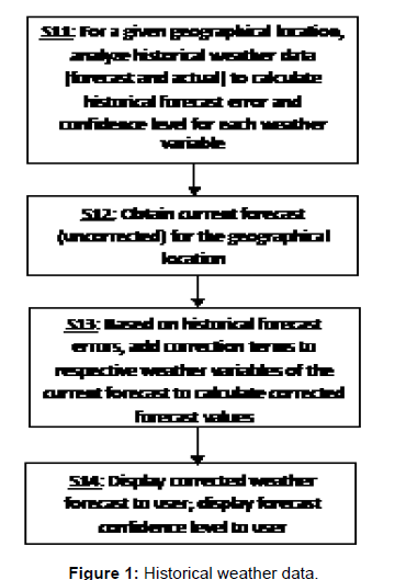
Figure 1: Historical weather data.
The current weather forecast for that geographic location is then obtained (step S12). The “current forecast” refers to the standard forecast that has not been corrected using historical data. Current forecast data may be obtained from, for example, NOAA or other weather forecast services. Then, for some or all weather variables in the current weather forecast, correction terms, which are the historical “actual minus forecast” value calculated in step S11, are added to the respective forecast values provided by the current forecast, to calculated the corrected forecasts for these weather variables (step S13). Each correction term may have a positive or negative value. The correction values depend on the geographical location and horizon period of the forecast, and may also depend on season.
For example, for most locations, for 6-day forecast of maximum daytime temperature, the mean of actual minus forecast value see Table 2 is less than 1 degree and therefore no correction term needs to be added.
In the case of probability of precipitation, on the other hand, a correction can be made to improve the accuracy of the forecast. For example, for Los Angeles, CA, if the currently forecasted probability of precipitation of a 3-day forecast falls within a range of 20%-50%, the forecasted probability should be corrected downwards significantly, e.g. the corrected probabilities of precipitation should be below 10% based on the result shown in Table 5. Analysis of historical data in the manner described in Section IV above can be performed for finer ranges of forecasted probabilities of precipitation (e.g., (20%, 30%), (30%, 40%), (40%, 50%)) to obtain the corresponding actual probabilities and the actual-minus-forecast values, which are then used to correct the forecast values.
As another example, corrections in quantitative precipitation can be meaningful for some locations. For example, for Seattle, WA, if a 3-day forecasted 24-hrs quantitative precipitation is 0.4 inches, then a correction of 0.27 inches will be added see Table 7, , resulting in a corrected 3-day forecasted 24-hrs quantitative precipitation of 0.67 inches.
As yet another example, for actual vs. 2-day forecasted wind speeds see Table 8, a correction term may be added when the forecasted wind speed is relatively high. For example, for Los Angeles, analysis of historical data shows that when the actual wind speed is 20-30 mph, the forecasts tend to under-forecast it by about 9 mph. Therefore, a correction term can be added when the forecasted wind is over a certain value. Further, additional analysis of the historical data can be performed to calculate the actual-minus-forecast wind speed value when the forecast value is within various ranges [10-20 mph, 20-30 mph, etc] so that appropriate correction values can be added based on the forecasted value.
The corrected weather forecast values calculated in step S13 are provided to a user (step S14). This step may be implemented in a webbased system such as a weather forecast website.
In addition, in the analysis step S11, statistical confidence levels for the various forecasts may be calculated (optional). As shown in our studies, the standard deviations of forecast errors can depend strongly on locations, horizon period of forecast and the magnitude of the weather variable. Adding confidence levels to certain weather forecasts [for certain locations] has the potential for improving the quality of the forecasts. In one implementation, standard deviations of the “actual minus forecast” values are used as an indication of the confidence level. For example, for a 6-day forecast of daytime maximum temperature, the standard deviation of actual minus forecast, see Table 2 may be used as the confidence level. Take Los Angeles as an example, =4.96 degrees, meaning that for 68% of the time, the actual temperature will be within ± 5 degrees (1 sigma) of the forecast value, and for 95% of the time, the actual temperature will be within ± 10 degrees (2 sigma) of the forecast value.
In an alternative implementation, a reliability score (similar to a FICO score) can be devised in place of the traditional statistics based confidence level instead.
The confidence levels for the weather forecasts calculated in step S11 are also provided to the user in step S14 (optional).
The methods described above may be implemented as a web-based weather forecast service.
1We selected mostly metropolitan cities as opposed to fixed distance grid points in order to make the geographical locations more recognizable.
2We use σ/ √N as an approximation for the sampling error of the mean, σ/ and √2N as an approximation for the sampling error of the standard deviation
3This is similar to the html formatted web content, which adheres to a set of rules so that they can be processed by a variety of browsers, except the weather data are in binary form.
4Wind related data files typically are the largest as the forecasts usually target more granular time periods due to the volatile nature of wind direction and speed.
5It took approximately 3 weeks to download all the data. To maximize throughput, we used an 8 CPU desktop machine, which allowed us to run 8 simultaneous download jobs in parallel.
6For most locations, we used the latitudes and longitudes of local weather stations if available.
7Although one does have the option of using nearest neighbor interpolation method as well
8Many of the results can be requested in Excel format for users to perform their own data manipulations. But for space considerations in this report, we won’t list a separate ranking table for each column in the same data set.
9Due to limitations on the total number of pages for this report, some results of this study have been omitted here. The full result set will be presented in another report.
10The full result set will be presented in another report.
11Which can also be viewed as the realized, or the measured probabilities.
12Due to size limitations on this report, we chose to include a set of unranked results along with a set of ranked results.
13There are considerable differences between regions, however. But due to space limitations of this report, a more comprehensive analysis of quantitative precipitation will be presented in a separate report.
14This is because sampling errors are typically estimated under the assumption of independence. But co-linearity will tend to introduce correlations among the data (typically in consecutive order) in the time series; therefore it has the tendency to under-estimate the true sampling error.
15It is possible that extremely strong winds could skew the mean of forecasted errors for some regions; therefore we chose to work with a speed range between 20-30 mph here as supposed to 20 mph and up.
| Location |  |
 |
 |
 |
Location | |
|
|
|
| Roseburg, OR | 4.56 | 0.11 | 10.35 | 4.17 | Merced, CA | 5.78 | -0.08 | 5.38 | 3.98 |
| Portland, OR | 6.18 | 0.41 | 10.2 | 5.79 | Reno, NV | 6.91 | 0.01 | 5.04 | 4.48 |
| Riverton, WY | 7.53 | 0.74 | 9.43 | 6.62 | Nashville, TN | 5.64 | -0.03 | 4.89 | 2.99 |
| Los Angeles, CA | 3.73 | -0.64 | 9.19 | 5.08 | Great Falls, MT | 9.87 | 0.64 | 4.86 | 4.43 |
| Seattle, WA | 6.85 | 0.44 | 8.64 | 4.72 | Wilmington, NC | 6.95 | -0.12 | 4.86 | 5.04 |
| John Day, OR | 5.97 | 0.16 | 8.54 | 5.55 | Bismarck, ND | 8.72 | 0.45 | 4.8 | 4.17 |
| Redding, CA | 5.24 | 0.43 | 8.4 | 4.48 | Warm Springs, VA | 7.49 | 0.08 | 4.61 | 4.3 |
| Santa Monica, CA | 5.53 | -0.22 | 8.1 | 5.2 | Baltimore, MD | 6.72 | 0.19 | 4.51 | 4.33 |
| Denver, CO | 7.98 | 1.18 | 7.91 | 5.61 | Dallas, TX | 8.73 | 0.14 | 4.47 | 4.2 |
| Pasadena, CA | 5.52 | -0.34 | 7.29 | 5.53 | Albany, NY | 6.59 | 0.1 | 4.38 | 4.13 |
| Charlotte, NC | 5.26 | 0.18 | 7.08 | 3.48 | Cincinnati, OH | 5.94 | -0.14 | 4.38 | 4.23 |
| San Jose, CA | 6.06 | 0.93 | 7.08 | 3.64 | Wichita, KS | 9.96 | 0.32 | 4.37 | 4.25 |
| Charleston, WV | 3.93 | -0.02 | 6.9 | 2.47 | Chicago, IL | 8.32 | -0.09 | 4.36 | 4.35 |
| Palm Springs, CA | 4.95 | -0.26 | 6.84 | 5.08 | Mobile, AL | 7.36 | 0.27 | 4.33 | 5.42 |
| Boise, ID | 6.43 | 0.04 | 6.66 | 4.71 | South Lake Tahoe, CA | 7.35 | 0.16 | 4.21 | 4.09 |
| Battle Mountain, NV | 5.56 | 0.12 | 6.54 | 5.01 | Flint. MI | 8.3 | 0.35 | 4.02 | 4.3 |
| Portland, ME | 6.83 | 0.39 | 6.47 | 4.88 | Sioux Falls, SD | 8.88 | 0.15 | 4.01 | 4.08 |
| Augusta, ME | 5.8 | 0.12 | 6.37 | 5.12 | Cleveland, OH | 8.89 | -0.1 | 3.87 | 3.93 |
| Idaho Falls, ID | 7.75 | 0.69 | 6.36 | 4.98 | Las Vegas, NV | 6.68 | -0.07 | 3.73 | 4.51 |
| Mammoth, CA | 7.59 | 0.5 | 6.04 | 5.32 | New York, NY | 8.4 | -0.29 | 3.73 | 4.06 |
| San Francisco, CA | 9.06 | 0.16 | 5.99 | 4.67 | Buffalo, NY | 8.58 | -0.16 | 3.71 | 4.28 |
| Salt Lake City, UT | 7.55 | 0.32 | 5.98 | 5.22 | Amarillo, TX | 11.59 | 0.13 | 3.66 | 4.54 |
| Little Rock, AR | 6.37 | -0.08 | 5.89 | 3.57 | Santa Fe, NM | 8.1 | 0.35 | 3.43 | 4.98 |
| Burlington, VT | 6.01 | 0.01 | 5.72 | 5 | Boston, MA | 9.26 | 0.24 | 3.43 | 3.97 |
| Jacksonville, FL | 6.02 | 0.08 | 5.66 | 6 | Milwaukee, WI | 7.53 | -0.09 | 3.33 | 3.51 |
| San Luis Obispo, CA | 6.85 | -0.25 | 5.65 | 4.76 | Atlanta, GA | 7.13 | 0.29 | 3.1 | 3.68 |
| Houston, TX | 6.79 | 0.07 | 5.59 | 2.5 | Flagstaff, AZ | 6.76 | -1.11 | 2.59 | 3.88 |
| Duluth, MN | 8.42 | 0.42 | 5.57 | 4.29 | Las Cruces, NM | 8.27 | 0.06 | 2.45 | 4.63 |
| Spokane, WA | 7.42 | 0.31 | 5.56 | 4.05 | Phoenix, AZ | 5.55 | -0.22 | 1.91 | 4.22 |
| St. Louis, MO | 7.15 | 0.01 | 5.41 | 3.44 | Miami, FL | 7.64 | -0.28 | 1.4 | 5.28 |
Table 8: Actual vs. 2-day forecasted wind speeds, as ranked by the mean forecast errors for days with high winds. Here is the mean of actual wind speed, is the mean of actual minus 2-day forecasted wind speed, and (, ) are the mean and standard deviation of actual minus 2-day forecasted wind speed for wind speed in the range of (20 mph, 30 mph).
17It is worth noting that the statistical models presented in this study cannot be substitutes for weather forecast models based on atmospheric sciences. One should expect that advances in atmospheric sciences will result in better and more accurate weather forecast models going forward. The method proposed in this paper can be set up using empirical weather data from a rolling time window of 4 years or so, as this time interval cannot be too short since some weather events such as heavy rains do not occur frequently in many geographical locations. Also, as mentioned earlier in this paper, methods proposed in this study cannot be easily applied to studies of forecast accuracies of extremely rare weather events such as floods that occur once every hundred years.