Research Article - (2025) Volume 13, Issue 1
This article introduces a theoretical framework investigating the impact of Relative Humidity (RH) on temperature variations in nature. Previously, an analysis relying solely on environmental thermodynamics governed by radiation and the Stefan-Boltzmann law, named the “dry model,” revealed a nocturnal cooling rate of approximately 0.9°C/h in low relative humidity conditions (<85%) across three distinct Brazilian forests within the Amazonian biome. However, this rate decreased notably when RH surpassed 85%, attributed to an additional heating effect resulting from the coalescence of water molecules in the air. In this study, a novel “wet model” is developed, integrating terms proportional to RH and its time derivative, under the premise that clusters of water molecules and latent heat crucially depend on the quantity of water molecules and intermolecular forces. The findings demonstrate a superior fit to the data using the proposed model, effectively capturing both the nocturnal temperature decline and diurnal variations. This advancement is significant as it underscores the importance of considering water molecule clusters in developing a more precise model to replace the current methodology.
Water molecules • Natural ecosystems • Humidity • Thermodynamic model • Temperature dynamics
Understanding the processes of energy and matter transfer between biosphere and atmosphere has been a subject of interest of science in the last decades, specially to better comprehend the response of forests and other ecosystems to the global climatic change and land use and also to improve agricultural techniques. However, despite the considerable evolution of the research in this field, some important uncertainties are also persistent. One of them is the non-balance energy closure. It is well known by a large reported literature that, when the energy fluxes are measured by the Eddy Covariance (EC) method, the sensible and latent heat fluxes are underestimated [1,2]. Efforts to explain the non-closure have been undertaken by several authors over the past decades. Some suggest that the issue stems from a scale problem, which carries significant consequences for the measurement and modeling of turbulent fluxes [3]. Others propose that the problem is linked to turbulence conditions, which affect the assessment of energy budget closure, among other factors [4]. Fluxes measured using the EC method suffer from unavoidable biases caused by the frequency response limitations of the EC system and data processing methods [5].
In studying ecosystems, energy balance is estimated by measuring four energy fluxes: Net Radiation (Rn), Sensible (H) and Latent (Le) heat fluxes and energy flux in the Soil (G) [6]. However, these quantities refer to different spatial volumes: The measurement of Rn is punctual-frequently accomplished in the top of a tower, while G is taken inside de soil and H and Le are related to a footprint covering a surface of thousands of square meters [7]. In the literature there is an absence of theoretical approaches on the energy density–instead of energy fluxes at each point in space.
Although the eddy covariance method is widely used in current research, it is not without limitations, especially in the precise measurement of latent heat flux. The method is based on a minimum of assumptions that are never strictly fulfilled. Certain mathematical procedures, such as high-frequency filtering and coordinate rotation, changes in meteorological conditions and/or sensor drift, contribute to turbulent changes in the data being perceived as trends or low-frequency changes. Trends contaminating the signal need to be removed by a suitable detrending method, but determining the best method for trend removal is not straightforward [8].
Another issue with the estimation made solely by the empirical method is the homogeneity in the distribution of water vapor in the measurement area. If there is heterogeneity, such as areas with different types of vegetation or surfaces, the results may be affected. To accurately measure latent heat flux, it is essential to consider the potential underestimation of the variation of water vapor concentration in the air (Cw). Cw is measured by an infrared sensor that emits an infrared beam at a specific frequency and, under adequate calibration factors, estimates cw based on water molecule absorption at this frequency. Through the covariation of cw and wind velocity, the method provides estimates of latent heat flux (Le) [9]. The method operates under the assumption that there are no clusters of few water molecules in the air, meaning all water molecules diffuse freely through the air. However, in cases where clusters of a few water molecules (e.g. two molecules) form, there will be a release of latent heat that the sensors may not detect. This discrepancy arises because one molecule liquid water absorbs infrared radiation at the sensor’s beam wavelength. Additionally, the absorption coefficients of liquid water and vapor in a peak are not significantly different [10]. Consequently, the sensors may not be sensitive to the formation of clusters, as it represents a situation of latent heat release. The same principle applies in the case of cluster dissociation with latent heat absorption.
In order to better understand this research problem, it is of fundamental importance a more precise approach on the environmental non-equilibrium thermodynamics. This means that it is fundamental to better understand the behavior of temperature, since this is one of the variables that holds the most information about environmental systems [11]. Unfortunately, the hourly behavior of temperature is still nowadays described by empirical relations [12-15] that do not emphasize the real physical processes occurring in biosphere atmosphere interaction.
This study introduces a model for the hourly variation of temperature, developed based on physical principles and presents experimental findings obtained from Brazilian ecosystems. Initially, the physical principles and a discussion on the limitations of flux measurements are outlined. Subsequently, the model is developed and applied to experimental data for analysis.
Beyond the global energy balance model
In the point of view of statistical thermodynamics, the formation of small clusters of water should not be impossible. If one considers that Boltzmann statistics rules out the dynamics of cluster formation, taking into account the energy equipartition theorem, the probability of constituting a double water molecule cluster is [16]:

Where ε is the bond energy, k is the Boltzmann constant and T is the environmental absolute temperature. 3 kT is the term of energy equipartition considering the translational, vibrational and rotational degrees of freedom. For T = 300 K, 3 kT is 1.2 × 10⁻²⁰ J. However, the value of ε is not known with precision since it is very difficult to be directly measured, but some researchs in the literature present approximate estimates. For example, it is reported that ε ≈ 4.8 kcal/ mol, which is equivalent to 3.3 × 10⁻²⁰ J [17]. By using the Lennard- Jones potential to describe the hydrogen bond, ε ≈ 4.9 × 10⁻²¹ J. Despite the great difference between these values, it is important to note that they are comparable with 3 kT, meaning that the energy bond of small clusters of water molecules is comparable with the kinetic energy of the molecules of water vapor at ordinary conditions. By substituting the two values above in the Equation 1, the probability of a double water molecule cluster is, respectively, 94% and 33%. This means that the formation of small clusters of water molecules is expected, at least during the night.
The recent study discusses water clusters and density fluctuations in liquid water using extended hierarchical clustering methods [18]. The study includes simulations at room temperature for various sizes of clusters, estimating both their geometric shapes and the binding energy between molecules. According to the article, small clusters exhibit optimal shapes, implying a subtle balance between hydrogen bond enthalpies and structural distortions. The energy of water clusters is defined as the sum of interaction energy between molecules in the clusters and is directly proportional to cluster size. Another interesting result is that as the number of molecules decreases, the number of clusters increases. Additionally, heating up can destroy large, low-energy clusters into small, high-energy ones due to increasing defects in the topological structures.
In another study, it is shown that the average energy of hydrogen bonds between H2O molecules in the formation of cluster associates with the formula (H2O)n is compiled as 0.1067 ± 0.0011 eV. As the energy of hydrogen bonds between H2O molecules increases up to -0.14 eV, the cluster begins to self-destruct. The ordering of water molecules into associates corresponds to a decrease in entropy due to the organization between molecules, resulting in a negative value for the Gibbs free energy.
During the day, substantially lower values than the above are expected, as photon absorption could lead to the dissociation of the clusters.
One way to try to evaluate the latent heat flux more correctly, considering the formation of small clusters of water molecules, is the mathematical modeling of temperature behavior in environmental systems. From a thermodynamic point of view, temperature is a variable sensitive to energy flows in natural systems. In addition, it is known that temperature is one of the variables that holds the most information about the thermodynamics of natural systems [19].
The approach adopted in this work starts from a basic model-the global energy balance model:
Which does not take into account the latent heat flux. Adding a term, ξ, corresponds to the influence of release or absorption of energy by coalition or dissociation of clusters of water molecules:
Where R is the net radiation flux, T the absolute temperature, t the time, ρ and cp are the air density and specific heat, σ is the Stefan- Boltzmann constant and α and γ are two constants, with dimension of extinction coefficients (m−1). It is important to note that Equation 2 and 3 do not represent fluxes, expressing the temporal variation of the energy density in a point in the air (Jm−3s−1). However, these equations should have a relationship with the equation of balance of energy fluxes:

Where H and Le are the sensible and latent fluxes, respectively and G the energy flux in the soil, which should be expressed in Jm−2s−1 or W/m2. It is also important to understand that equation 4 is not valid for a certain point of space because G exists only in the soil and the other variables in the air. Therefore, the terms of Equation 4 should be considered mean values of the fluxes in a vertical column with a unit horizontal area. Although Equation 4 represents average quantities and equation 2 and 3 are valid for a point in space, these last equations can give information about fluxes. This connection is established by the continuity equation:
Where Γ is the energy density and ∇ × Γ the energy flux. The left term corresponds to Equation 3 and, in conditions in which horizontal variations can be neglected, the right term corresponds to the vertical gradient of the fluxes. This means that information of the fluxes can be extracted from Equation 3, i.e., if the temperature can be well modeled, it is possible to obtain information about the fluxes independently of the infrared sensors.
The method is not quite equivalent to the Bowen ratio [20]. The idea is to extract information about the fluxes by temporal series of temperature by establishing theoretically a relationship between ∂T/ ∂t and the fluxes. To fulfill this purpose, it is necessary to compose a theoretical model for the temperature variation.
Study area and experimental data
Automated sensors were utilized to measure air Temperature (T), net Radiation (R) and Relative Humidity (RH) in three distinct Brazilian ecosystems: Deep forest, border forest and transitional forest, as shown in Figure 1. The deep forest measurements were taken at a height of 60 m from a tower located in São Gabriel da Cachoeira (0.15 N; 66.45 W), an area that remains largely unaffected by human activities within the Amazon Forest. The average annual rainfall in this location ranges from 3000 to 3500 mm. The border forest site, located in the Rebio-Jaru Reserve (61.56 W; 10.46 S), is characterized by a mean canopy height of 33 m. Despite being situated within the Amazon Forest; this site is close to agricultural zones (approximately 50 km away) with intensive anthropogenic activity. Consequently, the average annual rainfall in this location is considerably lower than that of the deep forest, at 2100 mm/y. In the transitional forest, measurements were taken from a 40 m tower situated in an ecosystem that lies within a region between the Amazon Forest and Brazilian savannah (Cerrado) in a farm located in the municipality of Sinop (55.19 W; 11.25 S). The mean annual rainfall in this region is 2000 mm/y and the ecosystem is characterized by distinct dry (June-August) and wet seasons (December-March), with an approximately 28 m high canopy.
Air temperature and humidity measurements were taken using psychrometers (HMP 35, Vaisala, Inc., Helsinki, Finland), while radiation measurements were obtained using CNR1 net radiometers (Kipp and Zonen, Bohemia, NY, USA). The averages of the three variables were generated every 30 minutes and stored in data loggers (Figure 1).

Figure 1. Research area showing the Brazilian states where the localities whose data are used in this study are located. Each locality is situated in a distinct biome to test the proposed model under different conditions.
The model
A previous analysis of time series of temperature and relative humidity measured in the nocturnal period at five different Brazilian ecosystems pointed out that the amount of water in the air has a direct and specific effect on the cooling rate of these systems: When the Relative Humidity (RH) is low (<85%), the cooling rate is closed to 0.9°C/h and this value is predicted by Equation 2 of the global balance. In addition, when the relative humidity is higher than 85%, the cooling rate decreases intensively, so that, for a condition with RH near 100%, the cooling rate is reduced in several orders of magnitude. This means that, at high humidity, the water in the air adds a heating factor that compensates the cooling due to infrared emission, i.e., the heat liberation due to water molecules coalescence compensates the cooling to infrared emission.
In this way, a model for temperature was developed in this work, considering a dependence with Radiation (R) and Relative Humidity (RH). RH was chosen instead of the concentration of water vapour molecules due two reasons: First, due to the above commented problems with the relative incapacity of the gas sensors to distinguish between independent water vapour molecules and small clusters; second, because RH is a variable closely connected to the transfer of thermal energy in the environment.
The dependence of the nocturnal cooling with RH, described above, suggests that in any theoretical approach aimed to model the nocturnal temperature in the Amazonian ecosystems, it must be considered a (positive) term expressing the fact that the higher is the RH the lower is the cooling rate. In this work, the results of considering a linear term are presented.
However, the measured time series of temperature reveals another type of dependence with RH. When the time derivative of RH is higher (in the case of an abrupt increase, for example), an additional cooling effect is present. In Figure 2, this effect is pictured.
In this figure, the time series of nocturnal temperature is plotted for three nights when the relative humidity exhibited an intensive increase. The data are plotted in comparison with the almost linear cooling rate of 0.9°C/h (black line), theoretically predicted in conditions of low humidity. It is observed that, when RH increases significatively, the cooling rate reaches values below 0.9°C/h. In this way, the model also must include a (negative) term proportional to the time derivative of RH.
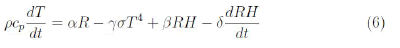
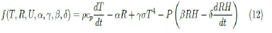
Therefore, the following model is attained in order to describe temperature:
Where ρ=1.184 Kg/m3 is the air density; cp=1012 J/Kg°C is the specific heat of the dry air; σ=5.67 × 10⁻⁸ Wm−2K−4 is the Stefan Boltzmann constant; R (W/m2) is the incoming solar radiation flux; T (K) is the air temperature; α and γ are two parameters given in m−1 adjusted with a dry model and β and γ are adjustable parameters related to the humidity and its derivative influence on temperature variation. The dimension of the equation is J/m3 (energy density).
The term on the left side of the equation represents the variation in sensible heat, while the first two terms on the right side correspond to the effect of radiation. Hence, the parameters α and γ represent the extinction coefficients of radiation in the air. To estimate the values of α and γ for the Brazilian ecosystems, data from a single ecosystem at intermediate latitude (Sinop) was used (Figure 2).

Figure 2. Nocturnal temperature feature (green) in conditions of high increase of relative humidity (red) in the transition forest in a night of October-2002 (top), June-2002 (middle) and Rebio-Jaru Forest in August-2008 (bottom). The linear approximation of temperature is the black line.
The last two terms on the right side of the equation were included based on the hypothesis of clusters with few water molecules. The latent heat critically depends on the number of water molecules that are bound together, which is determined by the binding energy that is proportional to the number of molecules. From the physical point of view, the terms depending on RH should be related with the intermolecular force between water molecules. Commonly it is described by the Lennard-Jones potential:
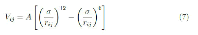
Where rij is the distance between the two interacting molecules and σ and A are constants. This expression can be rewritten as:
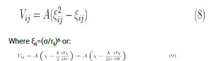
Where χ=ξ2, k=(∂ξ/∂r)−1 and considering a dynamical process of coalition/dissociation characterized by a mean velocity ν. This mathematical estimative points out that, if the interaction of the water molecules in the air is characterized by the Lennard-Jones potential, it is expected that the transference of energy due to latent heat is a process dependent of a couple of terms in which one is proportional to the variation rate of the other. In this way, the last two terms are directly connected to the intermolecular force between water molecules in the air. To obtain a more complete description, these two terms should be multiplied by the Probability (P) of two independent water molecules meet in the air, a quantity dependent on the mean number of molecules of water, which depends also on RH. But first of this, let us show the performance of Equation 6 in the description of the time series of temperature and, after this, introduce a factor representing P.
Computational fitting
In order to find the values of the coefficients in equation 6, a curve fitting that better fits this equation is performed. Curve fitting is a type of optimization that finds an optimal set of parameters for a defined function that best fits a given set of observations. It requires defining the functional form of the mapping function that maps examples of inputs to outputs, then searching for the parameters to the function that result in the minimum error. This provides the flexibility and control to define the form of the curve, where an optimization process is used to find the specific optimal parameters of the function. Once fit, one can use the mapping function to interpolate or extrapolate new points in the domain.
Error is calculated by using the observations from the domain and passing the inputs to the candidate mapping function and calculating the output, then comparing the calculated output to the observed output. Here, we used the non-linear least squares method of Levenberg-Marquardt (LM), an iterative nonlinear optimization algorithm that finds a local minimum (not necessarily the global minimum). It outperforms gradient descent and conjugate gradient methods for medium sized problems.
The primary application of the Levenberg-Marquardt algorithm is in the least-squares curve fitting problem: Given the empirical pairs (xi, yi) of independent and dependent variables, one need to find the parameters w of the model curve f (x, w) so that the sum of the squares of the deviations S(w) is minimized:
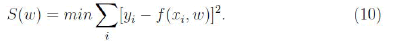
The function curve_fit of the scipy open source library of Python was used for curve fitting. The mapping function in this case will be:
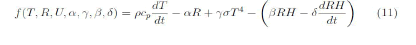
Where (T, R, RH) corresponds to the experimental input data and (α, γ, β, δ) to the remaining coefficients that must be optimized by a nonlinear least squares optimization process.
To test the model, time series of high quality temperature data corresponding to a month (approximately 1500 data points) were selected, which correspond to periods when the equipment was continuously operating. The chosen month was June for all three considered ecosystems.
The time evolution of temperature, humidity and radiation in the chosen time series is shown in Figure 3 for Sinop, Jaru and São Gabriel. The data in the first two locations is relatively stable, while in the third location it appears to have more measurement instability and fluctuations, which can be related to the presence of clouds inhibiting the radiation incidence and to the amount of rainfall in the area, which affects the measurements taken by the sensors.
Using the values of α=2.7 × 10⁻³ and γ=6.5 × 10⁻⁴ from the dry model, the curve fitting did not produce satisfactory results. As γ is connected to the emissivity and should not vary considerably, the effort to improve the fitting was focused on finding better values for α. Using the optimal values of α, the curve fitting was performed again to determine the values of β and δ. The comparison of these fittings with the experimental data is presented in Figure 4. The model fitting in the first two forests showed a satisfactory approximation to the data, although it couldn’t accurately reproduce the minimum temperatures. The third region experienced some instability, as described above, but the model still managed to capture the general behavior of the data well.

Figure 3. Experimental temperature, humidity and net radiation measured in Sinop (top), Jaru (middle) and São Gabriel (bottom) on the first seven days of June.
It is important to emphasize that the dry model reproduces a profile in which the temperature rises almost linearly during the day and decreases also almost linearly at night. Such behavior stems from the fact that the Stephan-Boltzmann constant, although proportional to the fourth power of temperature, is expressed in absolute scale (Kelvin), which has an almost linear behavior in the range of variation between 0 and 40°C. On the other hand, the wet model is capable of reproducing the correct curvature of the hourly variation of temperature, in which the second temporal derivative is negative during the day and positive during the night. However, the model fails to reproduce the daily minimum temperature values. As mentioned above, the model must take into account not only the intensity of intermolecular forces but also the Probability (P) of two water molecules encountering each other in the air. Therefore, we will modify the model by introducing P in the terms related to the influence of relative humidity:

Figure 4. Experimental temperature and the fittings using the wet model. For the probability P=1 of water molecules interaction (left), the coefficients obtained are α=1.05 × 10⁻³, β=2.4 × 10⁻³ and δ=179 for Sinop (top), α=0.55 × 10⁻³, β=2.7 × 10⁻³ and δ=154 for Jaru (middle) and α=0.2 × 10⁻³, β=2.7 × 10⁻³ and δ=191 for São Gabriel (bottom). Considering Equation 13 for the probability P of water molecules interaction (right), the coefficients obtained are α=1.55 × 10⁻³, β=2.3 × 10⁻³ and δ=385 for Sinop (top), α=0.9 × 10⁻³, β=3.0 × 10 −3 and δ=273 for Jaru (middle) and α=0.4 × 10⁻³, β=2.7 × 10⁻³ and δ=248 for São Gabriel (bottom); γ=6.5 × 10⁻⁴ was kept the same from the dry model.
As evidenced by a previous study, the dry model is capable of accurately reproducing the behavior of nighttime temperature when relative humidity is equal to or greater than 85%. This indicates that, for humidity values below this threshold, the presence of water in the air should not significantly modify local thermodynamics. Therefore, in this study, P was considered as a Heaviside type function with significant values (close to 1) only for relative humidity above 80%:
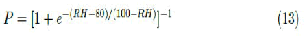
Taking into account this expression and equation 12, a new fit was performed for the same data. The results are shown in Figure 4.
It is worth emphasizing how the model fitting closely follows the temperature decay during nighttime, in contrast to the dry model, which resulted in a practically linear decay. This demonstrates the crucial role that relative humidity plays in determining nighttime temperature behavior. To better illustrate the comparison between the model and experimental data during the night, selected cases are presented in Figures 5 and 6. These cases were chosen specifically to highlight instances where the relative humidity reaches more than 85% or experiences significant fluctuations, in order to demonstrate the impact of the derivative term. The proposed model demonstrates an excellent fit with the temperature data, as evidenced by the close correlation in the plotted data in Figures 5 and 6. This supports the effectiveness of the model in describing the temperature behavior during the night.

Figure 5. The fittings of the nocturnal variation of temperature in June and October in Sinop with β=2.3 × 10⁻³ and δ=385. Red line: Relative humidity; black line: Experimental temperature; green line: Modeled temperature.

Figure 6. The fittings of the nocturnal variation of temperature in August with (a) β=3.0 × 10⁻³ and δ=273 in Jaru and (b) β=2.7 × 10⁻³ and δ=248 in São Gabriel. Red line: Relative humidity; Black line: Experimental temperature; Green line: Modeled temperature.
In conclusion, the study investigated the impact of relative humidity on the temperature variation in three different Brazilian ecosystems. The previous analysis, which only considered radiation and the Stefan Boltzmann law, revealed that the cooling rate was near 0.9°C/h when the RH was low but decreased significantly when the RH was higher than 85% due to the additional heating effect from the water in the air. To address this issue, a new model was developed incorporating terms proportional to RH and its time derivative, based on the hypothesis that clusters of water molecules and latent heat critically depend on the number of water molecules. The results showed that the proposed model provides a better fit with the data, even in the presence of fluctuations. However, further improvements are necessary to capture the local dependence of the adjustable parameters and include the relative humidity dependence on radiation. At night, the model effectively captured the temperature decay.
The authors would like to express their gratitude to Brazilian Coordenacao de Aperfeiçoamento de Pessoal de Nível Superior (CAPES) and Conselho Nacional de Desenvolvimento Cientifico e Tecnologico (CNPq) for supporting this study, as well as to thank the Large-Scale Biosphere-Atmosphere Program (LBA), coordinated by the National Institute for Amazonian Research (INPA), for the use and data availability, logistical support and infrastructure during field activities.
The authors have no relevant financial or non-financial interests to disclose.
Data will be made available on reasonable request.
[Crossref] [Google Scholar] [PubMed]
[Crossref] [Google Scholar] [PubMed]
[Crossref] [Google Scholar] [PubMed]
[Crossref] [Google Scholar] [PubMed]
Citation: Maionchi DO, et al. "A Model for Relative Humidity-Driven Temperature Dynamics in Natural Ecosystems". J Climatol Weather Forecast, 2025, 13(1), 1-6.
Received: 26-Mar-2024, Manuscript No. JCWF-24-30533; Editor assigned: 28-Mar-2024, Pre QC No. JCWF-24-30533 (PQ); Reviewed: 11-Apr-2024, QC No. JCWF-24-30533; Revised: 18-Mar-2025, Manuscript No. JCWF-24-30533 (R); Published: 25-Mar-2025, DOI: 10.35248/2332-2594.25.13(1).001-005
Copyright: © 2025 Maionchi DO, et al. This is an open-access article distributed under the terms of the Creative Commons Attribution License, which permits unrestricted use, distribution and reproduction in any medium, provided the original author and source are credited.