Research Article - (2025) Volume 13, Issue 1
Ensemble learning has drawn appreciable research attention attributable to its exceptional generalization achievement. In the field of rainfall prediction, many researchers have adopted various machine learning techniques based on varying meteorological parameters. This paper contributes to employing ensemble techniques for rainfall prediction based on seven climatic features form the Ghana meteorological agency covering 1980-2019 for 22 synoptic stations. The experiments involved 6 base algorithms (Logistic regression, decision tree, random forest, extreme gradient boosting, multilayer perceptron and K-nearest neighbor), 3 meta algorithms (Voting, stacking and bagging) and the ensemble learning. More specifically, the ensemble approach in this study focused on the combination of the base classifiers and vote meta classifier. The performance of the models was evaluated based on correlation coefficient, mean absolute error and root mean squared error. Another mode of comparison of the models was dependent on the time taken to build and test the models on the supplied test set. Generally, findings from the study showed that the ensemble learning outperformed both base and meta algorithms.
Base algorithms • Meta algorithms • Ensemble learning • Rainfall prediction
Artificial Intelligence (AI) has received much attention in this age of global digitalization which has yielded varying techniques and applications adapted in various aspect of our lives. Popular among these techniques, is machine learning that is being employed in many sectors. Machine learning has been extensively used in areas such as cyber security for intrusion detecting which remains a critical security issue [1]. In the medical field, conditions such as breast cancer early detection system, early diagnosis of Alzheimer disease which largely affects the elderly and the prediction of cardiovascular diseases have all received considerable attention from machine learning techniques. Generally, the performance of these machine learning techniques hinges on continual learning which is technically grouped under supervised learning and unsupervised learning [2].
Climate change analyzes the nature of the weather over a region for definite period of time [3]. One of the significant climate change burdens is the prediction of rainfall over a specific region by employing meteorological features such as humidity, temperature, wind speed and sunshine. In spite of the significance of rainfall prediction which aids in proper management of water resources, the relevance of the accurate and prompt prediction of this phenomenon is largely due to its severe impact on sensitive sectors of the economy such as agriculture, energy and the outcome of floods that goes on to destroy critical installations and livelihoods [4]. For instance, in, half a million people were severely affected by rainstorms across four African countries with about 500,000 people losing their lives due to flood events between 2007 and 2009.
Also, in view of the rainfall variability affecting agriculture within Sub-Saharan Africa, it has been reported, that malnutrition that led to the death of about 50,000 children could worsen. In relation to time, forecasting of the weather can be short range, medium range and long-range covering a duration of 48 hours, three to seven days and beyond seven days respectively. To accomplish a successful seasonal forecast is subject to a meticulous insight into the oceanatmosphere interactions. Further to this, an understanding of the influence of this interaction on seasonal rainfall prediction is based on the timescales such as monthly, bimonthly and seasonal that the ocean-atmosphere interactions span [5].
In spite of the use of state-of-the-art technology, rainfall predictions do experience some level of constraints due to the chaotic nature of the weather. Among various approaches to accurately predicting rainfall, machine learning techniques have received much attention by researchers. These include but not limited to decision tree, random forest, K-nearest neighbour, support vector machine and neutral networks. Variations among the performance of these algorithms suggests an adoption of an ensemble model that is achieved by assimilating different models. The thrust convention is to scale the various classifiers and merge them to yield an improved classification which surpasses the performance of the individual classifiers. It has been established that ensemble methods enhances prediction performance [6].
Over two decades, ensemble learning has been widely adopted due to the magnitude of its generalization. It has been well documented in many studies that multiple classifiers generally enhance generalization as compared to the individual classifiers. Fundamentally, two major steps are involved in building an ensemble scheme: (1) Construction of various base classification models; (2) Using an efficient technique to merge them. Generally, the merging algorithms could be achieved by voting and estimate weights. In spite of the fact that there isn’t an affirmed theory that explains how diversity enhances ensemble model accuracy, it has been well established that the prerequisite feature for an outstanding ensemble performance is the diverse and accurate nature of the base classifiers [7]. Therefore, in this paper, the major focus is employing ensemble methods to enhance rainfall prediction. In summary, the significant contributions we put forward in this paper are as follows:
• First, we conduct an empirical study of six base algorithm models and three meta algorithm models to predict rainfall.
• Second, we propose the utilizing of meta-classifiers as the combining technique for the ensemble framework to predict rainfall.
• Third, we demonstrate the necessity of employing evaluation metrics such as Correlation Coefficient (CC), Mean Absolute Error (MAE) and Root Mean-Squared Error (RMSE) to evaluate ensembles models.
The rest of the paper is as follows: Section II describes related work carried out in rainfall prediction; the methodologies employed for this current study is given in section III. Also, the results and discussion are presented in section IV and finally, section V constitutes the conclusions form this study.
Related research works
The ensemble methods have received much attention in various studies. To evaluate the performance of an ensemble model and base classifiers, undertook a study that firstly compared the individual performances of base classifiers and meta classifiers with an ensemble model built by the voting technique. Their study adopted the voting approach to merge three classification algorithms including random forest, random tree and J48 [8]. Findings from the study showed that the performance of the ensemble method surpassed the performance of the individual classifiers. The classification confidence of some base classifiers employed in an ensemble model has been investigated. According to, weighted voting which is reliant on classification confidence exceeds the performance of simple voting. However, their study revealed that to enhance the performance of the weighted voting ensemble, a significant technique that needs to be adopted is the ensemble pruning via ordered aggregation. Ensemble learning has also been employed in the detection of the chloride concentration levels in the river [9].
Two base classifiers including Multi-Layer Perceptron (MLP) and Stepwise-Cluster Analysis (SCA) were employed. Based on these two classifiers, the authors of this study proposed an ensemble model based on MLP and SCA. Based on evaluation measure such as RootMean-Square Error (RMSE), Mean Absolute Percentage Error (MAPE), Nash-Sutcliffe Efficiency (NSE) and R2, findings from the study showed that the ensemble model (MLP-SCA) outperformed the individual classifiers. Results of RMSE, MAPE, NSE and R2 yielded 11.58 mg/L, 27.55%, 0.90 and 0.90 respectively, demonstrated the competence of the ensemble in predicting high levels of concentrated chloride. Similarly, has developed an ensemble model to predict the concentration of surface chloride of marine concrete. In their study, a comparison was undertaken between a proposed ensemble model and the individual base models that constituted the ensemble learning. The individual classifiers were combined to form the ensemble model using the weighted voting techniques which yielded a high accuracy rate [10].
Landslide and wildfire within the southeast Asia region has been assessed using ensemble learning methods. Utilized three ensemble models to assess the vulnerability of the southeast to landslide and wildfire. Random forest, gradient boosting decision tree and adaptive boosting were the three ensemble models evaluated based on accuracy, precision, area under the Receiver Operating Curve (ROC/ AUC) and confusion matrix. Findings from the study showed random forest outperformed the other two ensemble models with an accuracy of 0.81, precision of 0.78 and AUC of 0.91. Similarly, in a study to predict slope stability has compared the performance of ensembles models and base classifiers. The study compared the performance of ensemble models such as Extreme Gradient Boosting (XGB) and Random Forest (RF) to support vector machine and logistic regression. Based on precision, recall and accuracy, the performance of the ensemble models (RF and XGBoost) exceeded that of the support vector machine and logistic regression in terms of training and testing of the data used revealing the dominance of ensemble models.
Further has proposed an ensemble model to uplift the accuracy level of seasonal rainfall forecast consisting of gene expression programming and multi-stage genetic programing. Results from their research demonstrated that the ensemble model proposed, maximized the accuracy of the seasonal forecast by 30%. An ensemble approach for an enhanced solar power generation forecast. They employed two key diversity techniques that is structural diversity and data diversity as well as a proposed ensemble model composed of machine learning and statistical hybrid model. Based on combination methods such as simple averaging approach, weighted averaging using linear approach, inverse approach and using non-linear approach. Findings from their study revealed that the proposed ensemble model gained higher accuracy level in comparison to the individual models.
In a case study of bay sedimentation, employed ensemble learning to predict heavy metal contamination. Their study compared the extreme gradient boosting, random forest, artificial neural networks and support vector machines. Performance evaluation based on coefficient of determination; the extreme gradient boosting obtained the highest value compared to the other classification algorithms. Validation of the models depicted extreme gradient boosting the least reduction in coefficient of determination, with a decrement of 7.99%. However, the decrement in R2 values for random forest, support vector machines and artificial neural network were 10.26%, 36.19% and 8.31% respectively.
Ensemble learning techniques have been evaluated for the prediction of solar irradiance. Their study first of all used base algorithms such as support vector machine, artificial neural network and decision tree. Based on a five-year meteorological data, the study compared the performance of the base classifiers to two proposed ensemble learning techniques; boosting and bagging. Findings from the study showed the boosting and bagging techniques performed well based on the root mean squared error and coefficient of determination values.
We used the following 6 methods as base classification algorithms. The criteria for the selection of these algorithms to create the rainfall prediction models was based on criteria utilized. The base algorithms were implemented by using Scikit-learn.
The base algorithms
Artificial neural network-multi-layer perceptron: Multi-Layer Perceptron (MLP) is a type of artificial neural network known the feed forward artificial neural network. Artificial Neural Network (ANN) has been one of the most extensively utilized machine learning algorithm. ANN is embedded with diverse kinds used by researchers for various studies. Among the various kinds of ANN, the Multi-Layer Perceptron (MLP) has been widely used in many research disciplines. For instance, in hydro-climatological studies, MLP has been used to document the relation between predictors and its associated predictands. Describes the MLP with features such as layers and neurons. The layers of the MLP are descried as follows;
• The input layer is the description of the first layer.
• The hidden layers are the layers centered in the middle.
• The output layer of MLP is known as the last layer.
Based on an activation function, to achieve the desired output, the hidden layers combines weights and bias terms with inputs. Using n number of inputs x=x1, x2, … xn and vector of weights wj=w1j, w2j, … wnj for a given node j. The simulated yj at the node j is given by;
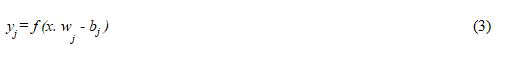
Where f(.) is the activation function, wj as the weight vector and the bias related to the node represented as bj
Therefore, the output is derived by:
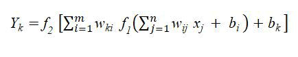
Where:
f1 and f2=Activation functions
J=Input layer
i=Hidden layer
k=Output layers
xj=Input
bi and bk=Bias relating to the hidden and output layers
m and n=Neurons in both the hidden and input layers
wij=Weights between the hidden and input layers
wki=Weights between the hidden and output layers
Yk=Output
K-Nearest Neighbour (KNN): K-Nearest Neighbour (KNN) which was first put forward by cover and hart in the prediction of textual problems. According to KNN performs comparatively well when the features employed in the model are few. The Euclidean distance for the KNN algorithm is computed by the equation below;
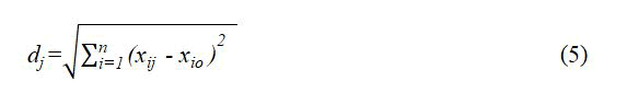
To calculate the KNN value, Equation 5 is used
Where:
xij=ith data point
xio=jth predictor
Zr=Predicted data
Zk=Neighboring data
Fk (dj)=Kernel function
Research has shown that the performance of the KNN hinges on the value of neighbors (K) employed. For the purpose of this current study, the value of K is 5 for all the training and testing.
Decision Tree (DT): Research has shown that the prominent algorithms employed in building Decision Trees (DT) include but not limited to Classification and Regression Trees (CART), C5.0 and Chi squared Automatic Interaction Detection (CHAID). Looking like the structure of a typical tree, decision tree consists of nodes, leaf and roots. C5.0 which is an improved version of C4.5, was utilized for the purpose of this current research work for the prediction of rainfall.
Random Forest (RF): Random Forests (RF) are robust ensemble classifiers originally introduced. In recent times, random forest has received much attention and chiefly in the domain of problems classified. Using this ensemble approach, random forest averages numerous decision trees to improve on the performance. Also, the ensemble technique deals with issues of overfitting and also exhibit proper handling of larger datasets; thus, convenient for this current study. The two main parameters in random forest are namely: Number of trees and number of variables. The number of weak learners employed is 100 and maximum depth tree of 16.
Extreme Gradient Boosting (XGB): Extreme Gradient Boosting (XGB) is an enhanced gradient boosting algorithm proposed and suitable for both classification and regression problems such as presented in the current study. XGboost has been widely used by researchers in machine learning and by data scientists chiefly due to its high-level execution time.
Logistic regression: Logistic regression is a classification algorithm that predicts the probability of instances based on a logit function. It operates on independent variables in generating binary output. Logistic regression best fit rainfall prediction scenario as a classification problem.
Base meta classifiers employed
Stacking: Stacking is a form of meta-classification proposed. It is an ensemble model that facilitates the combinations of prediction from base classifiers which serves as the new sets of training dataset for a final prediction by a meta-classifier.
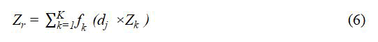
Staking, which is also considered as generalization of voting, generates a high accuracy in terms of predictions based on the combination of the output from the various models. Results from the base classifiers labelled as models 1, 2 and 3, are combined at the model labelled as trained model. The final output is therefore generated based on equation 7 below:
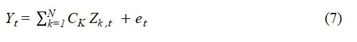
Where the output of the model K is represented by Zk,t for observation t with associated coefficients CK. The Scikit-learn library is utilized in the implementation of stacking.
Bagging: Bagging, which is also referred to as bootstrap aggregation is an ensemble learning method composed to handle both regression and classification problems, reduces variance and also prevents model overfitting. According to bagging can be viewed as model averaging method. Recently, researchers have not only demonstrated reduction in error of variance by bagging but also avoids increase in bias error. In view of its advantage of solving issues related to weak learners, a plethora of studies have adopted bagging as a consolidation factor among weak learners.
Voting classifier: A voting classifier is a machine learning model that operates by an ensemble approach of combining various models to make a prediction based on highest majority of voting. Voting serves as a folder of the various algorithms to exploit the distinctive nature of the individual algorithms. The predictions of the various models are averaged for classification purposes. Generally, the two types of voting the voting classifier supports are the hard and soft voting. In summary, to merge the predictions from diverse machine learning models voting classifier is imperative.
Datasets
The dataset employed for this study spans 1980 to 2019 and covers the entire country of Ghana. The data sourced from the Ghana Meteorological Agency (GMeT) includes rainfall, relative humidity at 3 pm and 6 am, wind speed, sunshine hours and temperature. The GMeT data is in accordance with the standards of the world meteorological organization. The datasets used for this study has seven (7) attributes covering the entire ecological zones of Ghana; i.e., coastal, forest, transition and savannah zones (Table 1).
| Climatic parameters | Units | Description |
| Maximum temperature | Degree celsius (°C) | Maximum temperature in degree celsius |
| Minimum temperature | Degree celsius (°C) | Maximum temperature in degree celsius |
| Rainfall | Millimeters (mm) | Rainfall amount recorded for the day |
| Relative humidity 0600 | Percentage (%) | Relative humidity at 6 am |
| Relative humidity 1500 | Percentage (%) | Relative humidity at 3 pm |
| Sunshine | Hours | Hours of sunshine in a day |
| Wind speed | Knot | Speed of the wind |
Table 1. Data description of climatic variables used for the study.
Test options
According to the results of implementing the selected classifier will be tested according to various test modes which includes percentage split, cross-validation, supplied test set and use training set. In the percentage split method, the evaluation of the classifier is based on how well it predicts an amount of percentage of data reserved for testing. Also, the cross validation employs a number of folds to evaluate the classifier. Furthermore, use training set approach involves evaluating the classifier on its performance with regards to the prediction of the class of the attributes trained.
However, this study adopted the supplied test set as the test option. This test options works by evaluating the classifier on how well it predicts the class of a set of instances. In all the datasets covering the four ecological zones of the study area, the instances were partitioned into a ratio of 70:30. Where the first part of the ratio which is 70 is used for training and the remainder of 30 is used for testing.
Ensemble combination approach and structure
Generally, the output of base classifiers are combined by largely two main approaches which is weighting and meta-learning methods. In this current study, the vote meta-combination was employed. With regards to the structure of the classifiers adopted for the ensemble, the parallel structure, which involves the combination of the output of independent base classifiers by a combination technique such as vote, was utilized.
Evaluation metrics
The efficiency of models has received varying approaches in many research works. In this current study, the evaluating metrics to assess the performance of the models includes Mean Absolute Error (MAE), Correlation Coefficient (CC) and Root Mean-Squared Error (RMSE). Especially, MAE and RMSE have been widely adopted in measuring predicted and actual values. The metrics are therefore detailed as follows:
Mean Absolute Error (MAE): Generally, mean absolute error describes the average prediction error. This evaluation metric has been employed in many studies evaluating the performance of models. For instance utilized MAE in a comparative study involving decision tree and artificial neural network. Recently employed MAE as an evaluation measure in study to analyze the performance of deep learning and machine learning algorithms for crop yield prediction. The value of MAE is estimated by averaging the predicted value and its correlative value (i.e., the actual value). MAE formula is shown in equation (8) below:
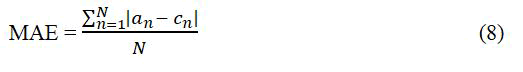
Where an represents the prediction value whereas cn is the expected value.
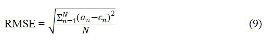
Root Mean-Squared Error (RMSE): Fundamentally, mean squared error is one of the most widely used measure for the prediction of observational values and predicted values of a model. Simply put, the root mean squared error is the square root of the mean squared error. Using Euclidean distance, RMSE shows the deviation of predicted values from actual values. According to rounding of RMSE and MAE improves accuracy prediction and waive the bias in model prediction.
Correlation Coefficient (CC): Correlation coefficient is the specific measure of the correlation between two variables. For the purpose of this study, the correlation between the actual and predicted values is measured. The actual mean method of the Karl Pearson correlation is employed for this study as shown below:
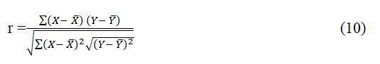
As utilized in the value of r is 1, the correlation is regarded as perfect. However, if the value of is 0, then there exists no correlation.
Execution time: The study as well employs time comparison approach to compare the performance of the models. This is done by comparing the execution time of the building and testing stages of the model on the supply test set as a tool to establish the efficiency of the various models.
Analysis of individual base algorithms and corresponding execution time
Tables 2 to 9, shows the performance of the base classifiers employed at the first stage of this study, and their corresponding training and testing times when tested on supplied test set. The performance of the classifiers evaluated according to mean absolute error, correlation coefficient and root mean squared error produce varying results.
| Algorithm | CC | MAE | RMSE |
| MLP | 0.8830 | 0.0961 | 0.2104 |
| KNN | 0.8341 | 0.1642 | 0.2422 |
| RF | 0.8102 | 0.1012 | 0.2311 |
| XGB | 0.8811 | 0.0804 | 0.3091 |
| DT | 0.8041 | 0.0641 | 0.3512 |
| LG | 0.8540 | 0.1540 | 0.2760 |
Table 2. Performance of base algorithms at the coastal zone.
| Algorithm | Training time (sec) | Testing time (sec) |
| MLP | 5.6 | 1.3496 |
| KNN | 0.1 | 0.0174 |
| RF | 0.3 | 0.3087 |
| XGB | 3.4 | 0.7185 |
| DT | 0.1 | 0.0262 |
| LG | 0.4 | 0.0349 |
Table 3. Base algorithms training and testing times at the coastal zone on supplied test set.
| Algorithm | CC | MAE | RMSE |
| MLP | 0.8698 | 0.1014 | 0.2201 |
| KNN | 0.8200 | 0.0721 | 0.3422 |
| RF | 0.8601 | 0.1103 | 0.2210 |
| XGB | 0.8214 | 0.0741 | 0.2710 |
| DT | 0.8312 | 0.1260 | 0.2264 |
| LG | 0.8518 | 0.1321 | 0.2317 |
Table 4. Performance of base algorithms at the forest zone.
| Algorithm | Training time (sec) | Testing time (sec) |
| MLP | 2.42 | 0.8993 |
| KNN | 0.10 | 0.0105 |
| RF | 0.30 | 0.7104 |
| XGB | 0.21 | 0.6203 |
| DT | 0.02 | 0.0159 |
| LG | 0.02 | 0.0329 |
Table 5. Base algorithms training and testing times at the forest zone on supplied test set.
| Algorithm | CC | MAE | RMSE |
| MLP | 0.8745 | 0.1914 | 0.2301 |
| KNN | 0.7802 | 0.1523 | 0.2814 |
| RF | 0.8714 | 0.1634 | 0.2605 |
| XGB | 0.8782 | 0.0821 | 0.2001 |
| DT | 0.7540 | 0.0726 | 0.2832 |
| LG | 0.7712 | 0.1285 | 0.2664 |
Table 6. Performance of base algorithms at the transition zone.
| Algorithm | Training time (sec) | Testing time (sec) |
| MLP | 2.04 | 0.2836 |
| KNN | 0.11 | 0.1149 |
| RF | 0.30 | 0.3994 |
| XGB | 0.21 | 0.5215 |
| DT | 0.20 | 0.0149 |
| LG | 0.12 | 0.0170 |
Table 7. Base algorithms training and testing times at the transition zone on supplied test set.
| Algorithm | CC | MAE | RMSE |
| MLP | 0.8411 | 0.0810 | 0.2291 |
| KNN | 0.7001 | 0.0628 | 0.2522 |
| RF | 0.8100 | 0.1110 | 0.2714 |
| XGB | 0.8711 | 0.1714 | 0.2136 |
| DT | 0.7014 | 0.1045 | 0.2315 |
| LG | 0.7112 | 0.1315 | 0.2840 |
Table 8. Performance of base algorithms at the savannah zone.
| Algorithm | Training time (sec) | Testing time (sec) |
| MLP | 3.02 | 2.1942 |
| KNN | 0.24 | 0.0320 |
| RF | 0.30 | 0.7432 |
| XGB | 0.20 | 0.2223 |
| DT | 0.01 | 0.0139 |
| LG | 0.02 | 0.0110 |
Table 9. Base algorithms training and testing times at the savannah zone on supplied test set.
According to the coastal zone results as shown in Table 2, it can be seen that artificial neural network-multi-layer perceptron has the minimum root mean squared error 0.2104, maximum correlation coefficient 0.8830 and the minimum mean absolute error 0.0761. Extreme gradient boosting comes in second after multi-layer perceptron as the classifier with the second highest correlation coefficient 0.8811, the highest root mean squared error 0.3091 and second less mean absolute error 0.0804. The third base classifier in terms of correlation coefficient is the logistic regression. Logistic regression had a correlation coefficient of 0.8540, came in with the second highest mean absolute error of 0.1540 and the second highest root mean squared error 0.276. Overall, the decision tree algorithm has the least correlation coefficient of 0.8041. Generally, comparing the base classifiers in terms of mean absolute error, correlation coefficient and root mean squared error at the coastal zone, reveals that the utmost accurate classifier in terms of correlation coefficient and root mean squared error is neural network-multi-layer perceptron whereas decision tree has the lowest mean absolute error. Similarly, in the forest zone as shown in Table 4, findings from the base algorithms show that neural network-multi-layer perceptron has the maximum correlation coefficient of 0.8698, the minimum root mean squared error 0.2201 and the third lowest mean absolute error 0.1014. Random forest came in second after neural network-multi-layer perceptron with a correlation coefficient of 0.8601 and the second less root mean squared error of 0.2210. With regards to correlation coefficient, logistic regression came in third with a correlation coefficient value of 0.8518. However, it has the maximum mean absolute error 0.1321 and the third biggest root mean squared error 0.2317.
Contrary to the coastal zone, k-nearest neighbor has the minimum correlation coefficient at the forest zone. Again, a comparison of the base classifiers at forest zone in terms of correlation coefficient, mean absolute error and root mean squared, puts neural networkmulti-layer perceptron ahead of the other base classifiers as the most accurate. Furthermore, results from the transition zone as it appears in Table 6, exhibits a move from the coastal and forest zones results discussed. Comparison among the base classifiers in terms of correlation coefficient, mean absolute error and root mean squared error puts the extreme gradient boosting with the maximum correlation coefficient 0.8782, the minimum root mean squared error of 0.2001 and the second lowest mean absolute error of 0.0821. However, neural network-multi-layer perceptron which earned the maximum correlation coefficient in the first two zones; coastal and forest, came in second at the transition zone with correlation coefficient of 0.8745, the second lower root mean squared error of 0.2301 and a mean absolute error of 0.1914. Random forest comes in third place after neural network-multi-layer perceptron as the third highest correlation coefficient of 0.8714, but it’s the second highest in terms of mean absolute error of 0.1634. At the savannah zone, as presented in Table 8, the best correlation coefficient of 0.8711 belongs to extreme gradient boosting, neural network-multi-layer perceptron comes in second with a correlation coefficient of 0.8410 and random forest places third has 0.8100 correlation coefficient. Tables 3, 5, 7 and 9, shows the build and test times of the base algorithms on supplied test set covering the various climatic zones. Overall, the outstanding performance of multi-layer perceptron, random forest and extreme gradient base classifiers compared to the other base classifiers across all zones is very much consistent with the findings. Further, it can be clearly established that throughout all the zones, the base classifier that takes the longest time to build a model is the neural-network multilayer perceptron. However, with regards to the time to test the model son supplied test set, the longest test time is dominated by random forest and extreme gradient boosting.
Analysis of individual meta classifiers
Tables 10-13, shows the individual performance of the Meta classifiers based on correlation coefficient, mean absolute error and root mean squared error. The classifier with the best correlation coefficient 0.8601 goes to stacking at the coastal zone as shown in Table 10. At the same zone, the worst correlation coefficient 0.8431 is associated to the voting classifier. With regards to mean absolute error at the coastal zone, stacking again had the lowest 0.1336. As presented in Table 11, the best correlation coefficient at the forest zone 0.8632 belongs to voting whereas the worst correlation coefficient 0.8307 resulted from stacking.
On the other hand, in terms of the mean absolute error at the forest zone, bagging had the lowest 0.1872. Table 12 shows the performance of the meta classifiers at the transition zone. Again, voting had the highest correlation coefficient 0.8459 whilst bagging came second with 0.8271. As in the previous ecological zones, bagging had the lowest mean absolute error 0.1015 at the transition zone. Table 13 shows the performance shows the performance of the classifiers at the savannah zone. As observed in the other zones, voting had the best correlation coefficient 0.8521. However, stacking came in second with a correlation coefficient of 0.8337 but the lowest mean absolute error of 0.1151.
| Meta classifier | CC | MAE | RMSE |
| Voting | 0.8431 | 0.1656 | 0.2486 |
| Bagging | 0.8522 | 0.1336 | 0.2667 |
| Stacking | 0.8601 | 0.2238 | 0.2402 |
Table 10. Performance of individual meta classifiers at coastal 0.1656 zone.0.2486.
| Meta classifier | CC | MAE | RMSE |
| Voting | 0.8632 | 0.1943 | 0.2445 |
| Bagging | 0.8445 | 0.1872 | 0.261 |
| Stacking | 0.8307 | 0.3420 | 0.3882 |
Table 11. Performance of individual meta classifiers at forest zone.
| Meta classifier | CC | MAE | RMSE |
| Voting | 0.8459 | 0.1396 | 0.2370 |
| Bagging | 0.8200 | 0.1015 | 0.2406 |
| Stacking | 0.8271 | 0.2641 | 0.3252 |
Table 12. Performance of individual meta classifiers at transition zone.
| Meta classifier | CC | MAE | RMSE |
| Voting | 0.8521 | 0.1603 | 0.2007 |
| Bagging | 0.7931 | 0.1266 | 0.2510 |
| Stacking | 0.8337 | 0.1151 | 0.2812 |
Table 13. Performance of individual meta classifiers at savannah zone.
A comparison between the individual meta algorithms in terms of mean absolute error, correlation coefficient and root mean squared error. A visual inspection at the coastal zone shows the correlation coefficient of the meta classifiers almost having them same value. However, a close observation coupled with the corresponding tables show stacking as having the best correlation coefficient 0.8601 and root mean squared error 0.2402. On the forest zone, that voting performed as the best in terms of correlation coefficient 0.8632 and root mean squared error 0.2445.
Contrary to the performance of stacking at the coastal zone, at the forest zone it didn’t perform well with a high root mean squared error of 0.3882. The meta classifiers at the transitional zone. It can be inferred that voting has the highest correlation coefficient 0.8459 and the lowest root mean squared error 0.2370. The comparison between meta algorithms at the savannah zone, exhibits voting once more as the best meta algorithm in both root mean squared error 0.2007 and correlation coefficient 0.8521. The remaining meta classifiers has high root mean squared error beyond 0.250.
Analysis of ensemble approach
Tables 14-17, shows the results of the ensemble models evaluated based on mean absolute error, correlation coefficient and root mean squared error. The ensemble models were constructed based on the combination of the various base classifiers and the meta vote classifier. These include Vote +2 algorithms (MLP and KNN), Vote +3 algorithms (MLP, KNN an RF), Vote +4 algorithms (MLP, KNN, RF and DT), Vote+5 algorithms (MLP, KNN, RF, DT and XGB) and Vote +6 algorithms (MLP, KNN, RF, XGB, DT and LG). The results from the ensemble approach shows it achieved better performance than the base and meta classifiers. In spite of the fact that the results of the correlation coefficient of the ensemble method appeared close, there are slight distinctions in their performance. At the coastal zone, Vote +4 algorithms earned the highest correlation coefficient of 0.8991, the lowest root mean squared error 0.144 and mean absolute error of 0.0728. Similarly, Vote +4 algorithms at the forest zone outperformed the other ensemble models, because it achieved the highest correlation coefficient of 0.8906 and the lowest root mean squared error of 0.2206. However, the Vote +4 algorithms at the forest zone has a mean absolute error of 0.1275. Table 16 compared between the various ensemble models employed at the transitional zone. The highest correlation coefficient and lowest root mean squared error is associated to Vote +2 algorithms. Vote +2 algorithms have a correlation coefficient of 0.8891 whereas the minimum root mean squared error stood at 0.2544. Meanwhile, the mean absolute error of Vote+2 algorithm at the transitional zone is 0.1321. Results from Table 17 shows Vote +5 algorithms outperformed the other ensemble model at the savannah zone, with the highest correlation coefficient of 0.8856, a root mean squared error of 0.2033 and mean absolute error of 0.1295.
| Meta-learning | CC | MAE | RMSE |
| Vote +2 algorithms | 0.8856 | 0.1293 | 0.2618 |
| Vote +3 algorithms | 0.8801 | 0.1231 | 0.3007 |
| Vote +4 algorithms | 0.8906 | 0.1275 | 0.2206 |
| Vote +5 algorithms | 0.8823 | 0.1398 | 0.2667 |
| Vote +6 algorithms | 0.8544 | 0.1677 | 0.2477 |
Table 14. Performance of meta-learning at coastal zone.
| Meta-learning | CC | MAE | RMSE |
| Vote +2 algorithms | 0.878 | 0.1331 | 0.2311 |
| Vote +3 algorithms | 0.893 | 0.1171 | 0.2169 |
| Vote +4 algorithms | 0.8991 | 0.0728 | 0.1445 |
| Vote +5 algorithms | 0.8766 | 0.1238 | 0.2677 |
| Vote +6 algorithms | 0.8841 | 0.1263 | 0.288 |
Table 15. Performance of meta-learning at forest zone.
| Meta-learning | CC | MAE | RMSE |
| Vote +2 algorithms | 0.8891 | 0.1321 | 0.2544 |
| Vote +3 algorithms | 0.8855 | 0.1324 | 0.2766 |
| Vote +4 algorithms | 0.8831 | 0.1266 | 0.2865 |
| Vote +5 algorithms | 0.8842 | 0.1287 | 0.2742 |
| Vote +6 algorithms | 0.8834 | 0.1285 | 0.2653 |
Table 16. Performance of meta-learning at transition zone.
| Meta-learning | CC | MAE | RMSE |
| Vote +2 algorithms | 0.8767 | 0.1375 | 0.2877 |
| Vote +3 algorithms | 0.8544 | 0.1368 | 0.2453 |
| Vote +4 algorithms | 0.8467 | 0.1287 | 0.2421 |
| Vote +5 algorithms | 0.8856 | 0.1295 | 0.2033 |
| Vote +6 algorithms | 0.8834 | 0.1343 | 0.2113 |
Table 17. Performance of meta-learning at savannah zone.
Analysis of ensemble methods time of execution on supplied test set
On zonal basis, the time taken to build and test the ensemble models on supplied test set are displayed in Tables 18-21. Generally, it can be deduced that Vote +6 algorithms at the coastal zone has the longest ensemble model build time of 24.08 seconds, while the shortest build time is 0.07 seconds at the forest zone belonging to Vote +2 algorithms. A careful look at the testing time of the ensemble models across the various zones shows that, Vote +5 algorithms at the forest zone had the longest test time of 4.78 seconds. Furthermore, the shortest test time can also be located at the same zone. The shortest test time to test the various models on supplied test set is 2.67 belonging to Vote +4 algorithms.
| Meta-learning | Training time (sec) | Testing time (sec) |
| Vote +2 algorithms | 0.09 | 3.08 |
| Vote +3 algorithms | 0.65 | 3.45 |
| Vote +4 algorithms | 2.56 | 3.67 |
| Vote +5 algorithms | 18.77 | 3.05 |
| Vote +6 algorithms | 24.08 | 3.22 |
Table 18. Ensemble method training and testing times at the coastal zone.
| Meta-learning | Training time (sec) | Testing time (sec) |
| Vote +2 algorithms | 0.07 | 2.98 |
| Vote +3 algorithms | 0.86 | 3.09 |
| Vote +4 algorithms | 3.67 | 2.67 |
| Vote +5 algorithms | 16.08 | 4.78 |
| Vote +6 algorithms | 19.78 | 4.53 |
Table 19. Ensemble method training and testing times at the forest zone.
| Meta-learning | Training time (sec) | Testing time (sec) |
| Vote +2 algorithms | 0.11 | 4.08 |
| Vote +3 algorithms | 0.59 | 4.44 |
| Vote +4 algorithms | 3.98 | 3.98 |
| Vote +5 algorithms | 12.98 | 4.43 |
| Vote +6 algorithms | 23.09 | 3.67 |
Table 20. Ensemble method training and testing times at the transition zone.
| Meta-learning | Training time (sec) | Testing time (sec) |
| Vote +2 algorithms | 0.67 | 3.86 |
| Vote +3 algorithms | 4.87 | 4.06 |
| Vote +4 algorithms | 7.56 | 3.62 |
| Vote +5 algorithms | 18.05 | 3.98 |
| Vote +6 algorithms | 20.56 | 3.75 |
Table 21. Ensemble method training and testing times at the savannah zone.
This paper proposes an ensemble approach to develop zonal based rainfall predictions models. Monthly climatic data sourced from the Ghana Meteorological service, for 22 synoptic stations in Ghana has been used. The dataset, which covered the period of 1980-2019 employed for the study consisted of predictors such as minimum temperature, maximum temperature, rainfall, relative humidity, sunshine hours and wind speed. Our comprehensive experiments led to the development of base algorithms models including logistic regression, decision tree, extreme gradient boosting, random forest, K-nearest neighbour and multi-layer perceptron. Also, the individual meta algorithm models employed includes bagging, stacking and vote and the ensemble models. These diverse models were evaluated by employing Correlation Coefficient (CC), Mean Absolute Error (MAE) and Root Mean-Squared Error (RMSE) as performance metrics. Also, to undertake a comparative analysis among the models, the time taken to build and test on the supplied test set was carried out. At the first zone, which is the coastal zone, ensemble approach Vote +4 algorithms (Multilayer perceptron, K-nearest neighbour, random forest and decision tree) produced the best results. Similarly, the best prediction accuracy at the forest was achieved by same ensemble approach (i.e., Vote +4 algorithms). Our results showed that, Vote +2 algorithms (Multi-layer perceptron and K-nearest neighbour) performed comparatively better at the transition zone for prediction. Lastly, the best prediction model at the savannah zone was based on the ensemble model comprising of vote meta classifier and five base classifiers namely multi-layer perceptron, K-nearest neighbour, random forest, decision tree and extreme gradient boosting. Generally, the findings from this study shows that the ensemble models performed best compared to the individual base and meta algorithms. Our results is consistent and complement findings from other previous studies which is therefore indicative the ensemble models is potent for rainfall prediction.
[Crossref] [Google Scholar] [PubMed]
Received: 18-Jul-2024 Editor assigned: 20-Jul-2024 Reviewed: 03-Aug-2024 Revised: 19-Jan-2025, Manuscript No. JCWF-24-33027 (R0; Published: 26-Jan-2025, DOI: 10.35248/2332-2594.25.13(1).001-010
Copyright: © 2025 Drah K, et al. This is an open-access article distributed under the terms of the Creative Commons Attribution License, which permits unrestricted use, distribution, and reproduction in any medium, provided the original author and source are credited.