Journal of Climatology & Weather Forecasting

Malawi, just like the rest of the world, is facing several challenges relating to climate change. Changes in precipitation are one of the problems that Malawi has been facing. Reduction in precipitation that the country has faced in some growing seasons led to scarcity of water (Population Action International and the African Institute for Development Pol- icy, 2012), which in turn led to food crisis. In 2001/2002 and 2004/2005 growing seasons about 2, 829, 435 and 5, 100, 000 Malawians, respectively, were affected by drought and food assistance was required [1]. In 2006 Malawi was forced to import food to distribute in the lean months of January to March due to 2004/2005 drought which affected food production [1]. The areas that are mostly hit by droughts are Karonga, Salima, Zomba, Nsanje, and Chikwawa [1]. Apart from droughts, Malawi is also frequently hit by floods, with the lower Shire being the most affected area. Droughts and floods leave no time for farmers to recover [2]. The frequency of floods and droughts has been increasing, with the number of individuals affected increasing too [2,3].

Changes in growing seasons that we are currently facing are due to climate change [2]. Growing seasons no longer start at the time they used to start [2]. We are also currently experiencing short growing seasons, which are characterized by prolonged dry spells [4]. Due to unpredictable changes in growing seasons, farmers are unsure of when to plant [2]. In a quest to increase production, farmers have resorted to expensive hybrid crops [2] making crop production expensive.

The drying up of Lake Chilwa in 1995/1996 and 2011/2012 [5], simply confirms that we are experiencing a different climate to what it used to be. Temperatures in the lower Shire were noticed to be increasing [6]. Change in temperature is one of the indicators of climate change. Climate change, specifically change in temperature, affects many aspects of aquatic life. For example, water temperature controls growth, development, and survival of cold-blooded animals [7]. Change in temperature, above or below the preferred range, is likely to lead to decrease in number of many aquatic organisms [8]. The rise in temperature has an effect on metabolism, life cycle, and behavior of some marine species [9]. The migration of fish and other species from shallow to deep waters (to areas where they can survive) is associated with change in temperature [8]. Change in water temperature is associated with many changes in the aquatic life, hence deep waters are considered to be good indicators of climate change. Deep waters are sensitive to changes of the environment [10].

Lake surface water temperature (LSWT) data, in form of remote sensing images, provided by the Arc lake Project are obtained through the use of satellites. Surface water temperature observations, within a lake, are obtained at various locations and for each location at different times (the data are obtained both spatially and temporally). Advanced along Track Scanning Radiometers (AATSRs) are used to derive these observations. With LSWT observations obtained at high frequency both spatially and temporally, the volume of data to handle is high. One of the ways through which computational burden can be reduced in this case is by approaching the data as functional data and transforming the data into principal components [11] principal components reduce the dimensionality of data by giving modes of variation that are dominant in the data.

Most climate data, for example LSWT, are characterized by periodicity due to annual effects. With the climate changing, there is a possibility that LSWT recordings of a particular location on a lake, for each specific time of the year, may not be similar for different years. Thus one of the ways through which climate change can be observed is by examining the periodicity in LSWT observations. Liu et al. [12] provides a method called principal periodic components (PPCs) that are capable of separating the components that explain the variability in the response into those that are nearly-seasonal and those that are not.

The purpose of this study is to find out whether there is any exact annual variation (component of LSWT that occur repeatedly each year/that is seasonal) in LSWT observations for Lake Malawi or not. Elements of climate such as precipitation, temperature and wind conditions have an influence on LSWT. We expect these elements to be periodic; hence their effect on LSWT should also be periodic. If there is no any exact annual variation in LSWT, then the elements of climate that affect LSWT are changing- which is an indication of climate change. LSWT observations for the study are remote sensing images which are processed into continuous data.

This study demonstrates one of the possibilities on the utilization of deep waters in carrying out climate change-related studies. Apart from looking at climate change using LSWT, this study looks at LSWT of Lake Malawi in relation to the lake being a home to biodiversity and a global heritage [13]. In the quest to protect biodiversity in Lake Malawi, there is a need to monitor the temperature of water which is an important component when it comes to survival of various living organisms in the lake- this paper addresses just part of such studies.

Data description

LSWT data for Lake Malawi is considered in this study. The data are provided by the Arc lake Project. The data are in form of remote sensing images which are then processed in to continuous data. The images were taken at a spatial resolution of one kilometer. Advanced along Track Scanning Radiometers (AATSRs) were used to derive these observations of lake surface water temperature. The observations were made at different locations within the lake, and at different times. We will consider monthly observations from January 1992 to December 2011 (228 months) in order to have only complete cycles for easy application of some of the techniques that will be used in the analysis. We have 1061 spatial locations whose time series are under consideration (Figure 1) shows these spatial locations.

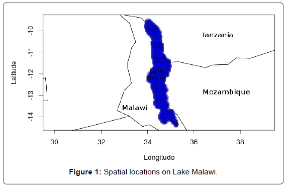
Figure 1: Spatial locations on Lake Malawi.

Bootsma and Jorgensen (n.d.) provide some details on Lake Malawi. Lake Malawi, which is the ninth largest lake in the world, the third deepest freshwater lake in the world, and a home to greater diversity of fish species than any other lake, is a global heritage. The lake contains about 7% of the available surface water and it covers an area of about 29, 500 Km², with a volume of about 7, 775 Km³. The maximum depth of the lake is about 700m, with a mean depth of about 264 m. The largest catchment area of the lake is in Malawi, followed by Tanzania, then Mozambique. The level of water on the lake is greatly influenced by precipitation and evaporation; hence it is likely to be affected by climate change. The benefits from the lake include fisheries, water for irrigation, transportation, and generation of hydroelectricity.

The surface temperature of water on Lake Malawi was obtained at high frequency both spatially and temporally, hence the volume of data is high. We will approach the data as functional data in order to reduce dimensionality- functional principal components (fPCs) and principle periodic components (PPCs) reduce dimensionality by giving modes of variation that are dominant in the data [14]. Since the data will be approached as functional data and we intend to study the periodicity in the data, the method of principal periodic components (PPCs) which is capable of separating variability in the data into that which is nearly periodic and that which is non-periodic will be used. The method also involves checking whether there is periodic variation in the data or not. The details for the method are provided by [12].

Data representation

Continuous observations collected at multiple times and assumed to be from a smooth process can be approached as functional data [15]. With functional data, an entire time series function is viewed as a single datum [14]. Given N time series each with T observations, the jth observation for the ith time series, yij , is represented in functional form as

(1)

ij s are errors which are assumed to have a 0 mean and a constant variance. xi (tij ) is the jth functional observation for the ith time series. Thus the ith time series is given as yi = xi (ti) + i. The functional curve xi (ti) is a linear combination of basic functions. With Φ (t) = (1, Φ1(t), Φ2(t), · · ·, ΦK (t)) a set of basic functions and Φj (t) the jth basis function,

(2)

With correlated data, both ordinary cross-validation and generalized cross-validation methods of choosing the smoothing parameter lead to under-smoothing [16] considering the relationship between λ and degrees of freedom, which are used to smooth the data, can be used in selecting the smoothing parameter in such a case. λ controls the degrees of freedom in the sense that increasing the smoothing parameter reduces the degrees of freedom, and vice versa [14]. λ and degrees of freedom are related in the following way:

(3)

Where S(λ) is the smoothing matrix and is given as

(4)

RL is the penalizing matrix.

Functional principal components (fPCs)

Functional principal components are used in summarizing variation in the data [15] they give the structure of variability in the data. fPCs, γi(t), define strong modes of variation by maximizing the variance

(5)

Subject to the constraints and with k≠d.

VARIMAX rotation described by Ramsay and Silverman [15] provides a separation between the most common modes of variation and those that are not common [14]. VARIMAX rotation is not capable of separating fPCs into those with strong annual periodicity and those without strong annual periodicity, hence we will adopt the method of principal periodic components (PPCs) described by [12]. Using a small number of fPCs to explain variability implies having less flexibility in explaining the variability [12] after rotating the fPCs, each fPC will have a higher variability to explain than if many fPCs were used [14]. On the other hand, using many fPCs, despite that it offers flexibility, means much concentration is put on individual time points [12], and each fPC has less variability to explain (after rotation).

Principal periodic components (PPCs)

The method of principal periodic components starts by defining benchmarks [12]. Given a vector of basic functions, fk with 1

12].

Consider U and V as rotation matrices on γ, vector of M fPCs, and f , vector of annual functions which are linear combinations of basic functions, respectively. The rotation matrices result from singular decomposition of the inner product of the spaces ΓM and FP .With utj the jth row of U and vt the jth row of V , the jth principal periodic component (PPC), ξj which is a rotated fPC, is given as

(6)

And the jth benchmark, θj which is the rotated annual function, is given as

(7)

Since we are trying to align the two functions in the same direction, the closeness measure can be looked at in terms of the angle between ξj and θj which is given as

(8)

Liu et al. [12] uses annual information (cumulative variation explained by benchmarks expressed as a proportion of the cumulative variation explained by PPCs) to separate the PPCs into those that are nearly-annual and those that are not. The annual information is given as

(9)

K and λk are the proportions of variation explained by the kth benchmark and PPC respectively. An elbow on the plot of annual information is used as a cut off. PPCs before the cut off are described as nearly-annual while those after the cut off are non-annual. Assuming nearly-annual variation and non-annual variation in the data, the curves can be decomposed as

(10)

Where 1 ≤ i ≤ N, N is the number of spatial locations; 1 ≤ t ≤ T, T is the number of times observations have been taken; m is the total number of nearly-annual and non-annual components; J is the number of nearly-annual components; K is the total number of fPCs (K = M in this case); μˆ(t) is the sample mean function;is the nearly annual part;Is the non-annual part; Part with components that explain a very small part of variation; are PPCs and scores of zi(t) (standardized time series curves) on ξj are given by where γ j are the fPCs; given by is the fPC score of on

Test for periodic variation

Liu et al. [12] provides a procedure for testing whether there is any exact annual variation in ΓM (space spanned by the M fPCs) or notwith the first PPC having a strong correlation (ρ1) with its associated benchmark, the procedure involves testing the null hypothesis that this correlation is 1, against the alternative hypothesis that the correlation is less than 1. That is:

H0: ρ₁ = 1, against

H₁: ρ₁ < 1. (11)

To formulate the null hypothesis, either M, the number of fPCs that span the space ΓM, or the percentage of variation to be explained can be fixed. The test involves checking if there is an intersection between leading fPCs and predefines Subspaces in the space that is nearly-annual [12].

In generating the null distribution for ρ1, data are slightly altered and least-favorable covariance is found- then bootstrap is applied. The hypothesized curves that are used to approximate the functional covariance under null hypothesis are given by

(12)

We set K to be the total number of fPCs and m the number of PPCs returned by PPCs method- 1≤i≤N and 1≤t≤T where N is the number of spatial locations and T is the number of times observations have been made at each spatial location. ξ1 is the first PPC. Given that the correlation between ξj and its associated benchmark is strong, the first PPC can be replaced by its benchmark θ1 and zi* is expected not to change much. Replacing the first PPC by its benchmark, we get the replacement curves

(13)

Bootstrap procedure is applied by sampling z˜i with replacement (and denote z˜b(tij ) as the results), and residuals obtained from pre-smoothing are also sampled with replacement (denoted ebij) to accommodate the effect of pre smoothing. The bootstrap curves and residuals are added (new observations are Wb ij = ~zb i (tij) + ^ebij with 1 ≤ b ≤ B where B is the number of times sampling has been done) and then re-smoothing is done. PPCs and first correlations are computed. The process is done several times. With the correlation between the first PPC and the associated benchmark not sufficiently large enough, Liu et al. [12] provides an approach for handling such a case. If the correlation between the first pair of the PPC and the benchmark is less than 0.05 critical value of the null distribution for ρ1, the null hypothesis is rejected in favour of the alternative hypothesis.

We are considering 1061 different locations on Lake Malawi on which LSWT observations were made. For each location, 228 observations were made. (Thus we have 1061 time series, each with 228 time points.) We are considering monthly observations from January 1992 to December 2011. The observations were taken in form of remote sensing images, and then processed into continuous data. The maximum temperature observed is 29.599°C and the minimum recording is 21.486°C (Figure 2) suggests that LSWT observations of a particular location on Lake Malawi, for each specific time of the year, are similar for different years- suggesting the presence of periodicity in the data. The figure shows that maximum temperatures on the lake are experienced around the months of September to April while minimum temperatures are experienced in the months of May to August in all years Malawi experiences a cool season from May to mid-August; a hot season is experienced from mid-August to November; the rainy season is experienced in the months of November to April. Thus the changes in LSWT from month to month can be attributed to change in seasons. With time plots in Figure 2 showing the presence of peaks and troughs, LSWT recordings may have periodicity. Despite LSWT observations of a specific time of the year being similar for different years (what seems to be strong periodicity in the data), the temperatures (for a particular time of the year on a particular location) seem not to be very similar for different years as observed from minimum and maximum temperatures through the years- the periodicity seems not to be strict.

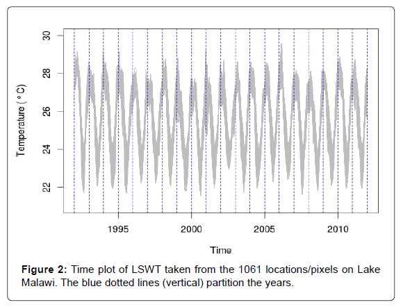
Figure 2: Time plot of LSWT taken from the 1061 locations/pixels on Lake Malawi. The blue dotted lines (vertical) partition the years.

We are looking at repeated measures of the same process (temperature). The observations are continuous and Figure 2 shows that LSWT observations for each location change smoothly. With these characteristics in mind, we represent the data in functional form. The time series for the various locations seem to share a sinusoidal shape. Thus we use Fourier basis to smooth the data. 229 functions are used (fitting a saturated Fourier basis), then we penalize the total curvature. A smoothing parameter, λ, of 10^-1 is used The focus of analysis is not on the overall mean and the total variability but on the direction of variation, hence we consider standardized time series [10] mean centering is done to remove vertical variation while dividing by the square-root of the variance makes the mean-centered time series have a variance of one. Figure 3 gives the standardized and smoothed time series.

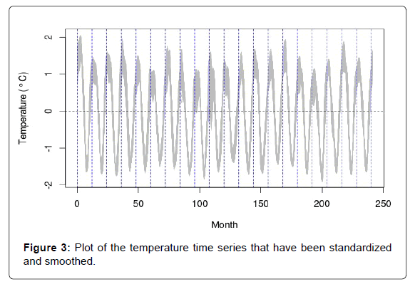
Figure 3: Plot of the temperature time series that have been standardized and smoothed.

We intend to apply the PPCs method on the LSWT data (standardized and smoothed LSWT time series) for Lake Malawi. We fix the number of fPCs, M, that span the space TM. We set M=166, we use a large number of fPCs in order to put much focus on individual time points since we are interested in the direction of variation. Using a less number of fPCs will offer less flexibility. Approximately 99.998% of variation in LSWT for Lake Malawi is explained by leading 166 fPCs (explained by the space T166). 229 Fourier basis functions are used to span the space of benchmarks. We have monthly observations from January 1992 to December 2011, thus the frequency is 20 and the period, P, is 12. Figure 4 gives the total variation explained by a specific number of fPCs and PPCs. The plot for fPCs (blue plot) simply shows the decrease in variation explained by fPCs as we move from one leading fPC to the next. The plot for PPCs does not have a clear sinusoidal shape (sinusoidal shape depicts the presence of periodicity) due to the large number of fPCs we have decided to keep. For a specific number of principal components, the variation explained by PPCs is much lower compared to that explained by fPCS which shows low annual variation.

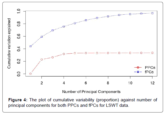
Figure 4: The plot of cumulative variability (proportion) against number of principal components for both PPCs and fPCs for LSWT data.

P=12 and M>P, hence the PPCs method used only the first 12 fPCs in ΓM and it (PPCs method) returned only 12 PPCs. Only the first 12 fPCs have associated bench- marks to compare to. The measure of periodicity for each PPC is provided by the co-relation between the PPC and the associated benchmark. The PPCs are arranged in descending order based on their periodicity. The correlations between the PPCs and their associated benchmarks are provided in Figure 5. For the first six PPCs, the co-relations between PPCs and their associated benchmarks are strong. The drop in correlations is noticeable after the sixth PPC. The strong correlations between the first six PPCs and their associated benchmarks suggest that there is periodicity in LSWT data for Lake Malawi. The periodicity is as a result of annual factors such as seasons. There are also PPCs with less strong and weak correlations with their associated benchmarks these PPCs suggest that LSWT for Lake Malawi is also affected by non-annual factors.

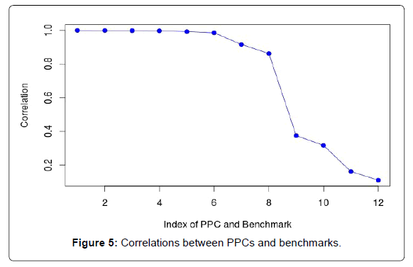
Figure 5: Correlations between PPCs and benchmarks.

Figure 6 shows 4 of the 12 PPCs together with their associated benchmarks. Plot of the first pair (Pair 1) which has the strongest correlation (approximately 0.999) among all the pairs shows that there is much resemblance between the PPC and its associated benchmark which is strictly periodic. There is also strong resemblance between the second and third PPCs and their associated benchmarks. For the first three PPCs, though there is much resemblance, there seem to be some slight departure from being strictly periodic. The twelfth PPC clearly departs from being strictly periodic.

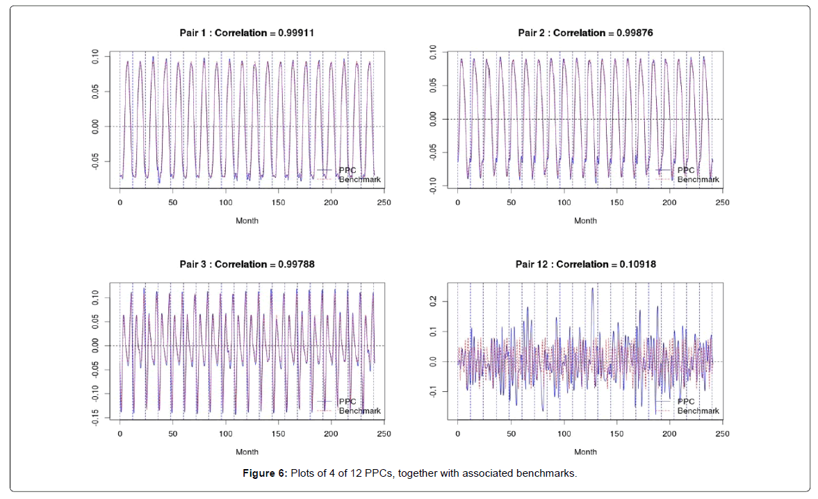
Figure 6: Plots of 4 of 12 PPCs, together with associated benchmarks.

Figure 7 (Scree plot), which is a plot of annual information (AI), separates the PPCs into those that are nearly annual and those that are not. There is a very sharp drop on how good the PPCs are at explaining annual variation in LSWT data for Lake Malawi after the sixth PPCthus the cut off is 6. In Figure 5 we also notice a slight big drop in correlation between PPCs and benchmarks after the sixth PPC. The first six PPCs are nearly-annual, while the rest (the other six) are nonannual. Thus there is strong annual variation (periodicity) in LSWT data for Lake Malawi (evidenced from the six PPCs which are nearlyannual). The six non-annual PPCs show that there are also non-annual factors that are making the data less periodic.

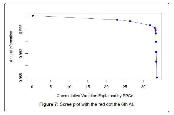
Figure 7: Scree plot with the red dot the 6th AI.

There are both nearly-annual variation and non-annual variation in LSWT data for Lake Malawi. Hence the LSWT curves for Lake Malawi can be decomposed into three parts- seasonal, unseasonal, and noise. Figure 8 gives plots of the noise (top plot) remaining after the effect of the 166 fPCs specified is removed; the middle plot gives the nearly- annual (seasonal) part of the data; while bottom plot gives the non-annual (unseasonal) part of the data. It Figure 8 shows that the patterns of LSWT time series for Lake Malawi are influenced by both annual and non-annual factors. By looking at the plots, a big proportion of variation is nearly-annual (annual factors have a great influence on LSWT).

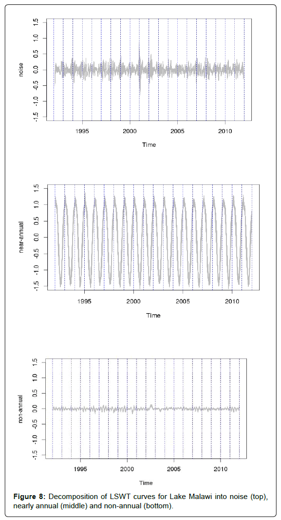
Figure 8: Decomposition of LSWT curves for Lake Malawi into noise (top), nearly annual (middle) and non-annual (bottom).

Given that the correlations between the first six PPCs and their respective benchmarks are strong (there is strong periodicity in LSWT data for Lake Malawi), we are interested in finding out whether there is/are any component/s in LSWT data that occur repeatedly each year (that is/are cyclic) or not we want to find out if there is any exact annual variation in T166. We follow the procedure described in Subsection 4.4. Despite that the periodicity in LSWT data for Lake Malawi is strong; Figure 9 shows that it is not strict. There are no components in the data that occur repeatedly each year. This could be as a result of climate change. With no any exact annual variation in LSWT data for Lake Malawi, we can conclude that LSWT for Lake Malawi is not strictly periodic.

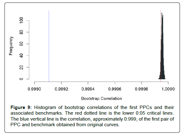
Figure 9: Histogram of bootstrap correlations of the first PPCs and their associated benchmarks. The red dotted line is the lower 0:05 critical lines. The blue vertical line is the correlation, approximately 0:999, of the first pair of PPC and benchmark obtained from original curves.

Both annual and non-annual factors affect LSWT on Lake Malawi. Annual factors have a stronger influence than non-annual factors- this may be the result of most elements of climate being strongly periodic. Climate change may also be a cause of lack of strict periodicity in most elements of climate, resulting in LSWT lacking strict periodicity. The study has not identified specifically which factors are annual and which ones are non-annual. Identifying and studying changes in such factors is important in combating climate change and protecting biodiversity. We propose future research work to consider looking into specific factors that affect LSWT. The study has also not looked into the direction in which the changes are taking if there are extreme temperatures recorded on the surface of Lake Malawi.

Despite that LSWT for Lake Malawi has strong periodicity, it (periodicity) is not strict. Thus LSWT recordings for a particular time of the year are expected not to be very similar for different years. This is evidence that the temperature that the aquatic life in Lake Malawi is exposed to is changing. There are many aquatic organisms in Lake Malawi whose survival, growth and development depend on the temperature of the water. An example of such organisms is the various species of fish in the lake. There are millions of Malawians whose everyday survival depends on fisheries as source of employment, food and raw material. Each of the species of fish (cold-blooded animals in general) in Lake Malawi has a preferred range of temperature. Many species are likely to die when the temperature of water gets outside their preferred range. If the temperature of water in the lake (LSWT) will keep changing, one day we will wake up only to find that the surface of Lake Malawi is covered by a carpet of dead fish- which is a blow to biodiversity and a nightmare to those whose livelihoods heavily depend on fisheries. Some fish species (cold-blooded animals in general) are already scarce in places where they used to be abundant.

LSWT or water temperature of the lake in general, is greatly influenced by the elements of climate. Thus most changes that happen to the climate also affect the aquatic life, making deep waters a tool that can be used in detecting and measuring climate change. There is no any exact annual variation in LSWT for Lake Malawi; hence the elements of climate that affect LSWT are changing which is an indication of climate change.

Human activities have been associated with much of climate change and deterioration of the environment. Lake Malawi has only been spared from the horrors faced by Mudi and Lilongwe rivers in Blantyre and Lilongwe respectively for the fact that no major towns and cities are close to the lake. If we are to save our biodiversity in Lake Malawi, we need to stop climate change. The temperature of water on the surface of Lake Malawi is changing, an indication that water temperature in the lake is changing- this is likely to affect the aquatic life, which in turn is likely to affect millions of people. Climate change is taking place in Lake Malawi.

The Commonwealth Scholarship Commission (CSC) the University of Glasgow, and African Institute for Mathematical Sciences (AIMS).