Research Article - (2013) Volume 1, Issue 2
Keywords: Indian future climate; PRECIS; Precipitation; Regional climate models; Temperature
Climate change is recognized as one of the most serious challenges facing mankind today [1]. Driven by anthropogenic activities, it is projected to be a direct threat to our food and water supplies and an indirect threat to world security. It is believed that increase in the concentration of carbon dioxide and other greenhouse gases in the atmosphere and consequent global warming will influence hydrological regimes and will have serious implications on water resources management [1]. Global climate models (GCMs) are fundamental tools for predicting future climate to enable developing a better understanding of climate change. At the regional scale, there is an urgent need for relevant, targeted projections of regional climate change [2]. There has been a rapid change in climate in response to human influences caused by local, national and global social, economic, industrial, and land use developments [1]. These changes continue to have impacts on different aspects of society, including health, agriculture, water resources, and energy demand. Therefore, it is important to investigate observed changes in the present climate so that future climate predictions can be validated and put into context. Most studies of national climate variabilities have been made using long term series of data from a small number of stations [3,4]. Also these studies concentrate on analysing data for one or two climate variables, usually temperature or precipitation. Rainfall, the principal input to freshwater systems, simulated in the available GCMs has certain uncertainties which have to be taken into account while using for impact assessments [2].
GCMs reconstruct important details of the climate at smaller scales (regional to local), but further downscaling is much needed. Hence techniques such as regional climate models (RCMs) and other downscaling methods have been developed [5]. RCMs are an effective method of adding fine-scale detail to simulated patterns of climate variability and change as they resolve better the local land-surface properties such as orography, coasts and vegetation and the internal regional climate variability better through improved resolution of atmospheric dynamics and processes [6]. A typical RCM grid is of the order of 0.44o to 0.44o, although some climate simulations employ smaller grids, usually only for a shorter temporal horizon of simulations [5]. Downscaled data from the RCM, PRECIS (Providing Regional Climates for Impacts Studies), has been validated extensively at both regional and catchment scales in different parts of the world, and represents the mean climate reasonably well [7,8]. In India, dynamical downscaling has been implemented by the Indian Institute of Tropical Meteorology, Pune using the RCM, PRECIS. This model has depicted the surface climate over the Indian region, particularly the summer monsoon precipitation, both in terms of mean and extremes reasonably well [9].
RCMs are generally run for a baseline period and the results are compared with observed values for the same period. Normally, PRECIS runs with 50km horizontal resolution for the present climate (1961- 1990) using different baseline lateral boundary conditions (LBCs) and for future scenarios (2070-2100) using the Special Report on Emission Scenarios of the Intergovernmental Panel for Climate Change. This research work focuses on the application of an RCM, PRECIS (Providing Regional Climates for Impacts Studies) for making projections of future climate (2071-2100) in the Chaliyar river basin in terms of rainfall and temperature in order to assess its likely impacts. Also, meteorological data, rainfall and temperature for the present period (1981-2010), were analysed to identify and study variabilities, if any, present in the data.
Emission scenarios
The Intergovernmental Panel on Climate Change (IPCC) published a new set of emission scenarios in the Special Report on Emissions Scenarios (SRES) [10] to serve as a basis for the assessment of future climate. Among all the SRES scenarios, four marker scenarios (A1, A2, B1 and B2) are often used [11]. The A1 and B1 scenarios emphasize ongoing globalization and project a homogeneous world, while the A2 and B2 scenarios lay emphasis on social, economic, and environmental development on regional and local basis and project a heterogeneous world. The A1 scenario family has been developed into three groups describing alternative directions of technological change in the energy system viz., AIFI (fossil intensive), A1T (non-fossil energy sources) and A1B (balance across all sources). In the case of A1B scenario, balanced is defined as not relying too heavily on one particular energy source, on the assumption that similar improvement rates apply to all energy supply and end-use technologies.
In this study, the projected changes in rainfall and temperature in the A2 and B2 are analysed. The A2 scenario projects high population growth and slow economic and technological development, whereas the B2 scenario projects slower population growth, rapid economic development, and lays more emphasis on environmental protection. Emission of green house gases (GHGs) and other gases and the driving forces were quantified in the Third Assessment Report of the IPCC [12] for use in climate simulations using General Circulation Models (GCMs).
PRECIS
The Hadley Centre for Climate Prediction and Research, with the sponsorship of the United Kingdom Department for Environment, Food and Rural Affairs (DEFRA), the United Kingdom Department for International Development (DFID) and the United Nations Development Programme (UNDP) developed a flexible RCM, PRECIS (Providing Regional Climates for Impacts Studies), to serve as a practical tool for making projections of national patterns of climate change and hence to estimate its possible impacts and to assess vulnerability. RCMs do not replace GCMs, but are powerful tools to be used together with GCMs in order to add fine scale detail to their broad-scale projections [6]. PRECIS is freely available for use by scientists from developing countries, priority being given to those involved in vulnerability and adaptation studies conducted by their governments, to be reported in National Communications to the United Nations Framework Committee on Climate Change. Adaptation decisions made for running PRECIS shall be based on a range of climate scenarios accounting for the large number of uncertainties associated with projecting future climate. National climate change scenarios can be created locally for use in impact and vulnerability studies using local knowledge and expertise. Carrying out this type of work at a regional level will lead to much more effective dissemination of scientific expertise and awareness on assessing climate change impacts [13].
PRECIS is a hydrostatic, primitive equation grid point model with 19 levels described by a hybrid vertical coordinate system [14]. The version of PRECIS used in this study has a horizontal resolution of 0.44°×0.44° [15]. The model domain is so selected that a sufficiently large area is covered so that synoptic and mesoscale circulations generated within the RCM are not undesirably damped. Simultaneously, the chosen domain shall be sufficiently small so that the deviation of the large scale seasonally averaged circulations predicted by the RCM from the driving Atmosphere Ocean General Circulation Model is not overwhelmingly large to imply a significant perturbation to planetary scale divergent circulation. These are necessary to ensure consistency between the RCM solution and the pre-determined GCM solution external to the RCM domain [6].
The anticipated adverse impacts of projected climate change are of paramount importance in planning future development and utilisation strategies in the water resources and agricultural sectors. Simulations employing climate models under scenarios of increasing greenhouse gas concentrations and sulphate aerosols indicate marked increase in both rainfall and temperature over India in the 21st century. According to the downscaled climate projections by PRECIS for the Indian peninsula, an average temperature increase of about 1°C in winter and 2°C in summer and an average decrease in precipitation by about 10-20% are predicted. The decrease in precipitation is not uniform throughout the year; a decrease of up to 10% in spring, and between 10 to 15% in autumn, is likely to occur, whereas an increase of about 10-20% in winter is also predicted [9]. The predicted change in rainfall under the B2 scenario is relatively less than that under the A2 scenario. There are substantial spatial differences in the projected changes in rainfall. The maximum expected increase in rainfall (10 to 30%) occurs over central India. There is no clear evidence of any substantial change in the year-to-year variability of rainfall over the next century [9]. Surface air temperature shows comparable increasing variabilities in the A2 as well as B2 scenarios. The temperatures are projected to increase by as much as 3°C to 4°C towards the end of the 21st century. The warming is widespread over the country and relatively more pronounced over the northern parts of India [9]. Overall, these variabilities point towards increased concentrated precipitation events and longer drought spells. The changes are not uniform across the sub-continent too; the sharpest reduction in precipitation is predicted in the southern region, while small areas in the north might have a small increase in precipitation [9].
Study area-Chaliyar river basin
The Chaliyar is the fourth longest river in Kerala with a length of about 170km. The geographical area of the part of the river basin in Kerala is 2530km2 it lies between latitudes 11°06’N and 11°36’N and longitudes 75°48’E and 76°33’E. Figure 1 presents the Chaliyar river basin in Kerala along with its location in the PRECIS domain. The main river starts from the Elambalari hills at an altitude of 2,067m above mean sea level (MSL). The climate in the basin is typically that of humid tropics [16]. Meteorological data including daily rainfall, temperature, relative humidity and solar radiation at the Kottaparamba observatory of the Centre for Water Resources Development and Management (CWRDM), Kunnamangalam, Calicut were collected for the period 1981 to 2010. From the analysis of the rainfall data, it is observed that the southwest monsoon (June to August) contributes about 60% and the northeast monsoon (September to November) contributes about 25% of the annual rainfall respectively. The remaining 15% is received as pre-monsoon showers during the months April to May. December to March is the driest period. The average annual precipitation in the basin is 3012.61mm and the maximum and minimum temperatures are 34°C and 24°C respectively. The annual average relative humidity ranges from 60% (minimum) to 90% (maximum) in summer; the corresponding values for winter are 65% and 85%.
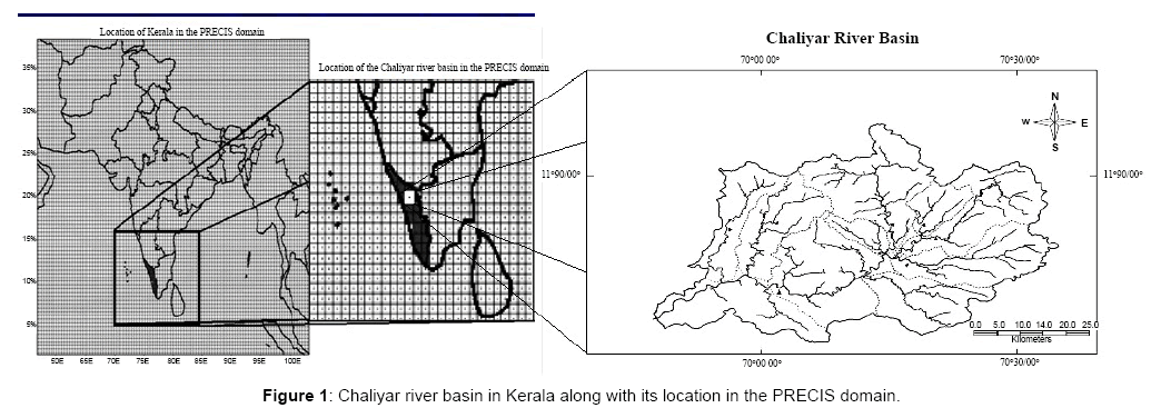
Figure 1: Chaliyar river basin in Kerala along with its location in the PRECIS domain.
Downscaling climate data using PRECIS
PRECIS was run with a horizontal resolution of 0.44° x 0.44° for the baseline period (1981-2010) using different baseline lateral boundary conditions (LBCs) and for a future period, 2071-2100, for the scenarios A2 and B2 outlined in the SRES of the IPCC [10]. The model was forced at its lateral boundaries by the results of simulations of a highresolution global model (HadAM3H) with a horizontal resolution of 3.75° x 2.5°. HadAM3H is an atmosphere-only GCM derived from the atmospheric component of HadCM3, the Hadley Centre’s state-of-theart coupled model which has a horizontal resolution of 3.75° longitude by 2.5° latitude. The Indian Institute of Tropical Meteorology (IITM), Pune, in collaboration with the United Kingdom Hadley Centre for Climate Prediction and Research has developed future scenarios for India [9]. The data generated in transient experiments by the Hadley Centre for Climate Prediction, United Kingdom, at a regional climate model resolution of 0.44° x 0.44° latitude by longitude grid points was obtained from IITM, Pune. Climate data for both A2 and B2 scenarios were collected and utilized in this study. The Chaliyar river basin having a drainage area of 2530km2 falls in one grid of 0.44° x 0.44° in the PRECIS domain. The downscaled climate data, collected from IITM, used in this study are precipitation and temperature (maximum and minimum) for the period 2071 to 2100.
Uncertainties associated with the projected climate data
There exist uncertainties in the projected climate change data collected from IITM, Pune. These uncertainties must be taken into account when assessing the impacts, vulnerability and adaptation options. However, all aspects of these uncertainties cannot be quantified yet [1]. There are inherent uncertainties in the key assumptions about and the relationships between future population, socio-economic development and technical changes that form the basis of the IPCC SRES. The imperfect understanding of some of the processes and physics in the carbon cycle and chemical reactions in the atmosphere generates uncertainties in the conversion of emissions to concentrations. Many things pertaining to the working of the climate system are not clearly understood yet, and hence uncertainties arise because of our incorrect or incomplete description of key processes and feedbacks in the model. This is clearly illustrated by the fact that current global climate models, which are based on different representations of the climate system, project different patterns and magnitudes of climate change for the same period in the future when using the same concentration scenarios. Climate varies on time scales of years and decades due to natural interactions between the atmosphere, ocean and land, and this natural variability is expected to continue into the future.
Bias correction of PRECIS predictions
A problem with the use of regional climate model output directly for hydrological purposes is that the computed precipitation and temperature differs systematically from the observed precipitation and temperature [17]. Bias is defined as the time independent component of the error [17]. Bias arises because of several reasons. It has a high spatial component as well. Also, the biases in the output subsequently influence other hydrologic processes like evapotranspiration, runoff, snow accumulation and melt [18-21]. Some form of pre-processing is necessary to remove biases present in the computed climate output fields before they can be used for impact assessment studies [22-24].
Several studies have been carried out on correction of bias in RCM output. In the simplest formulations of bias correction, only the changes in a specific statistical aspect of the computed field are used. Often the change in mean value or the variance is employed. This is equivalent to correcting the observations with an additive or multiplicative constant. Hay et al. [25] made use of the gamma distribution to match the distribution of modelled daily precipitation with that of observed daily precipitation. After bias correction, the corrected data can be used for stream flow simulations using a semi-distributed hydrologic model. It was observed that the corrected precipitation data did not have the day-to-day variability which was present in the observed data set. Apart from the bias in the computed precipitation, the estimation of flow suffers from the limited length of the RCM simulations (usually no longer than 30 years). Extrapolation of the distribution of computed discharges is then needed to estimate the extreme flood quantiles if the hydrological model is run directly with the RCM output. Leander and Buishand [20] applied a power law transformation to correct for the coefficient of variation (CV) and the mean of the precipitation values. They found that a relatively simple non-linear correction, adjusting both the biases in the mean and its variability, leads to better reproduction of observed extreme daily and multi-daily precipitation amounts than the commonly used linear scaling correction. This method of bias correction does not correct for the fraction of wet and dry days and lag inverse autocorrelation. A marked improvement was achieved with nonlinear transformation, adjusting the mean as well as the coefficient of variation of daily precipitation.
For this reason the method developed by Leander and Buishand [20] for bias correction was used in this study to correct for bias in temperature and precipitation data. The temporal and spatial resolution at which bias correction is applied is extremely important. In this study, this was performed at a temporal resolution of one day over a grid size 50km × 50km. Bias correction was performed on the downscaled PRECIS data for the period 1981-2010 (30 years). The most important statistics (coefficient of variation, mean and standard deviation on a scale of 5 days of the PRECIS data) were matched with corresponding quantities computed from the observed values. The daily precipitation P is transformed to a corrected value P* using:
 (1)
(1)
where a and b are constants.
The effect of sampling variability was reduced by determining the parameters a and b for every five-day period of the year [20]. Determination of the parameter b was done iteratively, so that the coefficient of variation of the daily precipitation values predicted by PRECIS matches the coefficient of variation of the observed daily precipitation. The coefficient of variation thus becomes a function of parameter b according to:
CV (P) = function(b) (2)
where, P is the precipitation in a block of 5 days (total of 73 blocks x 30 years = 2190 blocks). After evaluating the parameterb , the transformed daily precipitation values are calculated as:
P* = Pb (3)
Thereafter, the parameter a was determined such that the mean of the transformed daily values of precipitation matched with the observed mean. The parameter a depends onb . Parameter b depends only on the coefficient of variation and is independent of the value of parameter a . The values for a and b determined by this method for the A2 scenario were 0.1506 and 1.0344 and the corresponding values for the B2 scenario were 0.1679 and 1.1062. For correcting daily temperature, a different technique was used. Correction for temperature involves shifting and scaling to adjust the mean and the variance [20]. The corrected daily temperature T* is given by:
 (4)
(4)
where TU is the uncorrected daily temperature from PRECIS, TO is the observed daily average temperature (from the meteorologic data), TM is the corresponding daily average temperature obtained from PRECIS and SD is the standard deviation. Again both the statistics, the coefficient of variation and the mean, were determined for each 5-day block of the year separately.
Variability in annual and seasonal rainfall
A consistent decrease in annual rainfall was observed from 4159.90 mm in 1981 to 2724.20 mm in 1990. From 1990 to 1998, there was an increase in annual rainfall (up to 3585.80 mm). Again a decreasing inter-annual variability was observed till 2003 as the annual rainfall value reduced to 2536.60 mm. This was followed by a period that showed an increasing change in annual rainfall. The annual rainfall in 2006 was 2998.73 mm. This was followed by a decreasing variability till 2009. The annual rainfall in the year 2010 was 2691.94mm. The pattern which is observed in the variation of rainfall with a period of decreasing variability followed by one of increasing variability in annual rainfall is shown in Figure 2.
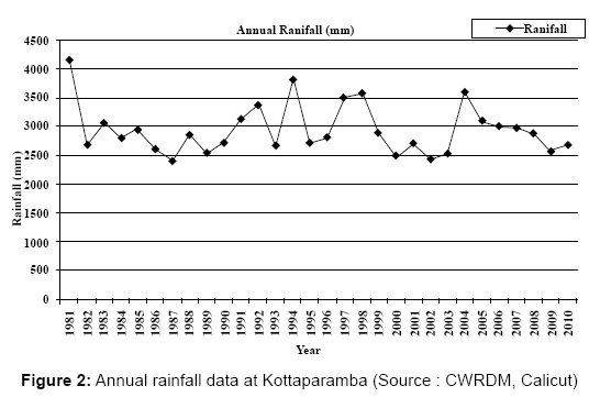
Figure 2: Annual rainfall data at Kottaparamba (Source : CWRDM, Calicut).
Rainfall during the southwest monsoon (June-September) also showed variability similar to that of annual rainfall. The average rainfall during this period was 2245.70 mm (1981 to 2010). The rainfall during this period was 3360.90 mm in the year 1981 and 2213.60 mm in 2010. The northeast monsoon rainfall (October-December) showed a slightly increasing variability. The average rainfall during this season over the 30 year period was 434.92mm. Northeast monsoon sets in the first week of October and retreats by the start of December. Except during the year 1986, which was a dry year, rainfall during this season was close to the average value in most of the years. The rainfall during this period was 570.40 mm in 1981 and 478.34 mm in 2010. The results of the analysis of rainfall during these seasons are presented in Figure 3.
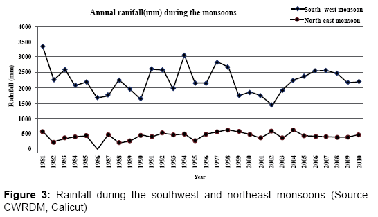
Figure 3: Rainfall during the southwest and northeast monsoons (Source : CWRDM, Calicut).
After studying the rainfall data during the southwest monsoon, it is observed that rainfall during the months of June and July showed a declining variability whereas this variability is not seen in the rainfall during the months of August and September. A seasonal shift in the rainfall pattern is observed with a significant decrease in southwest monsoon rainfall in recent years where as an increase in rainfall is observed during the northeast monsoon. Rainfall decline is more predominant in the months of June and July but not so in August and September. The decreasing variability in southwest monsoon rainfall over Kerala is supported by other researchers [16,26]. The decline in frequency of the weather systems in recent years over the peninsula may be an important reason for the reduction in southwest monsoon rainfall over Kerala. In addition to this, there is a drastic change in the biophysical resources of Kerala due to human interventions in recent decades [16]. It indirectly affects the physical processes in the earthatmosphere continuums and influences the distribution of local rainfall during winter and pre-monsoon seasons.
Variability in annual temperature
Analysis of temperature data reveals that, the average maximum temperature in the basin is 31.99°C and the average minimum temperature is 23.70°C. Figure 4 presents the annual average maximum and minimum temperatures in the Chaliyar river basin during the period 1981-2010. The average maximum temperature during the period 1981 to 1985 is 31.28°C, 1986 to 1990 is 31.90°C, 1991 to 1995 is 32.01°C, 1996 to 2000 is 32.11°C, 2001 to 2005 is 32.62°C and from 2006 to 2010 is 32.65°C. The corresponding values of average minimum temperature are 23.52°C, 23.61°C, 23.71°C, 23.78°C, 23.79°C and 23.89°C. From the above analysis it can be observed that there is a steady increase in temperature in the basin; the increase in maximum temperature is higher when compared to the increase in minimum temperature. Figure 5 is a plot of the average monthly temperature, average monthly maximum temperature and average monthly minimum temperature computed from the temperature data for the period 1981 to 2010. The maximum temperature is the highest in the month of April; the average value for the study period is 34.54°C. This is followed by the month of March with an average maximum temperature of 34.35°C. The lowest value of average minimum temperature is observed in the month of January (21.16°C) followed by the month of December (21.25°C). During the southwest monsoon season, the highest average maximum temperature is 29.67°C and the lowest average minimum temperature is 23.46°C. The corresponding values for the northeast monsoon season are 31.80°C and 22.60°C.
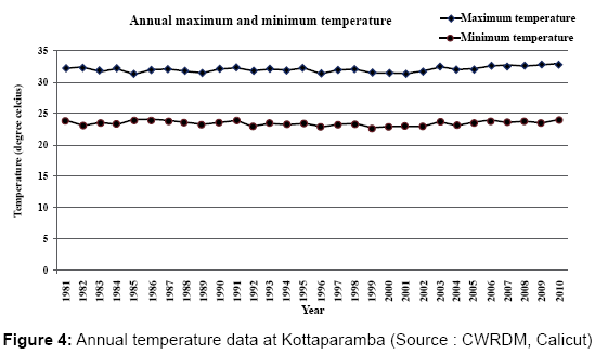
Figure 4: Annual temperature data at Kottaparamba (Source : CWRDM, Calicut).
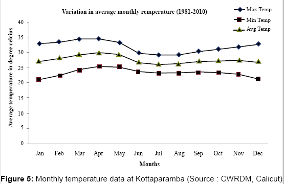
Figure 5: Monthly temperature data at Kottaparamba (Source : CWRDM, Calicut).
Analysis of the bias corrected temperature and precipitation data
The meteorologic data (precipitation and temperature) for the post climate change period, obtained from PRECIS was corrected for bias. The bias corrected precipitation and the bias corrected temperature for the future periods (2071-2100) along with the observed values are presented in the Figures 6 and 7 respectively. The projected annual rainfall in the Chaliyar river basin shows a decrease of about 20-25% from the present day annual average value in the A2 scenario. In the B2 scenario, the decrease was of about 10-15%. Annual average temperature shows an increase of about 3.3°C and 1.8°C from the present day values in the A2 and the B2 scenarios respectively. The maximum temperature increased by about 3°C and 2°C from the present average values in the A2 and B2 scenarios respectively. An increase of 3.5°C in the A2 and 2°C in the B2 scenarios was observed in the case of the minimum temperature.
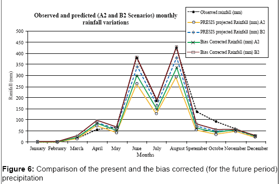
Figure 6: Comparison of the present and the bias corrected (for the future period) precipitation.
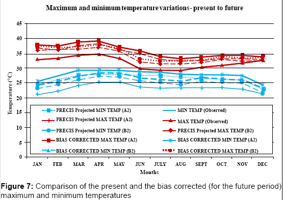
Figure 7: Comparison of the present and the bias corrected (for the future period) maximum and minimum temperatures.
In the A2 scenario, during the southwest monsoon period, an increase in temperature of 2°C and reduction in rainfall by 11.50% from the present day average values was observed. An increase in temperature of about 1°C and decrease in rainfall by about 8.79% was observed in the B2 scenario. Similar variabilities were seen in the northeast monsoon period also. In the A2 scenario, a decrease in rainfall by about 8.70% and an increase in temperature by about 2°C from the present day average values were observed. In the B2 scenario, it was observed that there was an increase in temperature of about 1°C and a decrease of about 4.73% in rainfall. In summer (pre-monsoon period), precipitation showed an increase of about 1.60% from the present day average value; the corresponding value in the B2 scenario was about 1.40%. The average temperature showed an increase of about 3°C and 2°C from the present day average values in the A2 and B2 scenarios respectively.
Climate change is expected to modify the frequency, intensity and duration of extreme events in many regions [24]. It is impossible to attribute single extreme events directly to anthropogenic climate change because of the probabilistic nature of these events. Also, there is always a chance that a given event may be the result of natural climate variability, even though an event of such magnitude has never been recorded [27]. It is clear that a dynamic downscaling experiment would have greater value if boundary conditions from more than one global climate model are used.
The potential changes of the surface climate over the Chaliyar river basin based on a single grid value from the 0.44o × 0.44° resolution PRECIS simulation driven by a high-resolution global model (HadAM3H) has been examined in this study. Results of simulations using the regional climate model, PRECIS for the present period and likely future climate were analyzed to develop an understanding as to how climate extremes may change in the Chaliyar river basin. The analysis was performed using the output from PRECIS after correction for bias. Bias correction was performed to ensure that important statistics (coefficient of variation, mean and standard deviation) of the downscaled output matched the corresponding statistics of the observed data. This method of bias correction does not correct for the fraction of wet and dry days and lag inverse autocorrelation. But, it was observed that a relatively simple non-linear correction, adjusting both the biases in the mean and variability, leads to better reproduction of observed extreme daily and multi-daily precipitation amounts. A marked improvement was achieved with a nonlinear transformation, adjusting the mean as well as the coefficient of variation of daily precipitation. The general results of this analysis can be incorporated into water resources management plans for the future in order to ensure sustainable water use in the river basin.