Biological Systems: Open Access

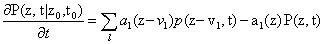
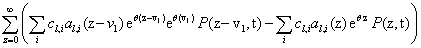
Simulating the behavior of gene regulatory networks is a formidable task for several reasons. At this level of description, only a few molecules (maybe dozens or hundreds) of each species involved in the regulation process is present, and this fact limits the possibility of considering the process as deterministic, as is done very often in most chemical applications. Here, the concept of con-centration of the species does not make sense [1,2]. On the contrary, under some weak hypotheses the system can be considered as Markovian, and can be consequently modeled by the so-called Chemical Master Equation (CME) [3], which is in fact no more than a set of ordinary differential equations stating the conservation of the probability distribution function - pdf -P in time:

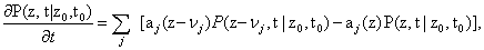
Where p(z,t | z₀, t₀) represents the probability of being at a state in which there are a number of molecules of each species stored in the vector z at time t when we started from a state z₀ at time t₀. a_j represents the propensity (i.e., the probability) of reaction j to occur, while v_j represents the change in the number of molecules of each species if reaction j takes place. This change is given, of course, by the stoichiometry of the reaction at hand.

What is challenging, however, in this set of equations is that they are de-fined in a state space which possesses as many dimensions as the number of different species involved in the regulatory network. Under this framework, if we consider N different species, present at a number n of copies, the number of different possible states of the system is n^N. This number can take the astronomical value of 10⁶⁰⁰⁰ if we consider some types of proteins, for instance [3]. This phenomenon is known as the curse of dimensionality in many branches of science.

To overcome this diffculty, most of the authors employ Monte Carlo-like algorithms (the so-called stochastic simulation algorithm, SSA [3-5].

However, Monte Carlo techniques need for as many as possible individual realizations of the problem, leading to excessive time consuming simulations, together with great variance in the results.

Separated representations involved in the Proper Generalized Decomposition described below allow circumventing the issues related to the high-dimensional character of the CME as was successfully proved in our former works discussed later. However, and despite the fact of being able to solve the CME, its solution requires a significant amount of computation, and thus, the simulation of a variety of scenarios remains a challenging issue because its computational complexity. For alleviating such a computational complexity an appealing route consists of calculating the moments of the probability distribution function instead of the pdf itself. Moments constitute a valuable description of great interest in many practical applications and then moment-based descriptions represent an appealing alternative to pdf-based descriptions. However, as discussed later, when deriving the equations that govern the time evolution of the pdf-moments, usually the one related to a moment of a certain order depends on higher-order moments and so-on. In order to close the model at a certain order, we must approximate higher order moments as a function of the ones lower or equal to the one considered. Such an approached constitutes the closure-based description.

As discussed later different closures has been proposed however, no closure relation is general enough to represent any possible scenario with the required accuracy. In this paper we propose using the expensive but very accurate CME solution efficiently obtained by invoking the PGD technology for fitting empirical polynomial closures. These closures are then used for obtaining moment-based solutions in an efficient way, because the integration of the evolution equations governing the time evolution of these moments can be performed almost in real-time, for scenarios that slightly differ from the ones that served to construct the empirical closure relation.

In any case it is important to note that the validity and accuracy of the computed closure-based solutions is never assured but in many cases is a valuable tool for pre-analysis. As soon as the main tendencies are obtained using the fast closure-based simulations, by performing a lot of simulations, all them very fast, finer analysis can be performed by solving the CME in a few selected scenarios of special interest extracted from the previous fast closure-based simulations.

Proper generalized decomposition for alleviating the curse of dimensionality

Dealing with the problem of the curse of dimensionality in a very different context, the authors presented in a previous work a technique that is now known under the name of Proper Generalized Decomposition (PGD) based on the use of separated representations [6,7]. Essentially, to avoid the exponentially growing complexity of the problem with the number of state space dimensions, the method approximates the variable of interest, say u, as a finite sum of separable functions:

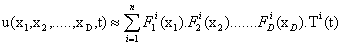
The reason for this particular choice motivated the method itself that is conceived as a greedy algorithm that computes one sum at a time and one product at a time, within a fixed-point, alternating directions algorithm. This leads to a sequence of one-dimensional (lowdimensional, in general) problems, one for each function Fⁱ _j that can be solved using your favorite technique (finite elements, finite volumes, finite differences, colocation, ...).

If M nodes are used to discretize each coordinate, the total number of PGD unknowns is N×M×D instead of the MD degrees of freedom involved in standard mesh-based discretization’s. Moreover, all numerical experiments carried out to date with the PGD show that the number of terms N required to obtain an accurate solution is not a function of the problem dimension D, but it rather depends on the regularity and separability of the exact solution as well as on the solution constructor itself. The PGD thus avoids the exponential complexity with respect to the problem dimension.

A PGD approach to gene regulatory networks simulation

The PGD approach to the problem of effciently simulating gene regulatory networks begins by assuming that the probability of being at a particular state z at time t can be approximated as a finite sum of separable functions, i.e.,

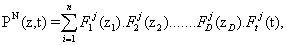
Where, as mentioned before, the variables zi represent the number of molecules of species i present at a given time instant. This particular choice of the form of the basis functions allows for an important reduction in the number of degrees of freedom of the problem, N × nnod × (D + 1) instead of (n_nod)D, where D is the number of dimensions of the state space and nnod the number of degrees of freedom of each one-dimensional grid established for each spatial dimension. For this to be useful, one has to assume that the probability is negligible outside some interval, and therefore substitute the infinite domain by a subdomain [0,….,m-1]^D, m being the chosen limit number of molecules for any species in the simulation. A similar assumption is behind other methods in the literature, such as the Finite State Projection algorithm, for instance [3].

Another important point to be highlighted is the presence of a function depending solely on time, F_t ^j (t). This means that the algorithm is not incremental. Instead, it solves for the whole time history of the chemical species at each iteration of the method. If one then assumes that n terms of the sum given by equation (3) are already known,

and look for the n + 1-th term, by substituting Equation (4) into the CME, Equation (1) gives a non-linear problem in 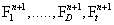that is solved by means of a fixed-point, alternating directions algorithm [8,9].

The separated representation just considered does not involve any assumption. Any solution defined in a high-dimensional space can be written, if it is regular enough, in a separated form if the number of terms in the finite sum decomposition is high enough. A polynomial of any order is no more than a sum of functional products, each depending on a different coordinate. Thus, solutions can be approximated with the desired accuracy by using a separated representation and an adequate constructor as the one described above.

Moments-based descriptions

Even if the use of separated representations allows circumventing the curse of dimensionality the computational cost remains considerable. This fact motivated in many other disciplines the replacement of the pdf by some of its moments [10-13], since many times the last suffice for having a view rich enough on the dynamics of the systems. The use of moment-based description was of major interest in different areas of statistical mechanics and it is being the more and more considered as an alternative to the discretization of the CME.

A moment represents the expected value of a random variable, z, raised to a certain power. An “expectation” is a specifically defined function in statistics, 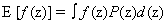when in continuous spaces or Σf(z)P(z) in discrete spaces. In general, we can talk about the i^th moment as:

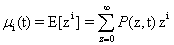
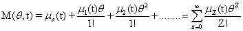
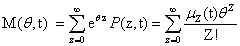
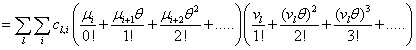
A probability distribution is uniquely defined by its full set of moments. Having access to these moments could eliminate the need to solve for the full distribution, depending on what information would be considered important. A special function, called the Moment Generating Function, is specifically in-tended for this purpose:

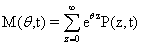
By taking the Taylor expansion of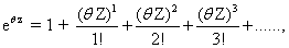 we can see the moments emerging from this function, the i-th moment associated with the i-th power of θ:

The following equations will be used extensively in the following derivation, so it will be useful to define them now:

From the Chemical Master Equation to moments based descriptions

Since we will be uniquely considering the structure of the Chemical Master Equation, we would like to derive a general version of the Moment Generating Function which can be used for any system. The CME for l reactions with stoichiometric change vl is:

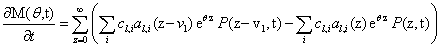
As we will see later on, the kind of rate laws associated with the system dramatically impact the complexity of the overall problem. We begin with the simplest case of kinetic mass action laws, following the derivation from Gillespie [10]. However, we would eventually like to take rational rate laws, such as Hill functions, as is seen in Milner et al. [14]. An example of a mass action rate law is 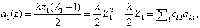where the law can be rewritten as a sum of coefficients c_l,i and variables a_l,i. This expanded, polynomial form will be exploited in our derivation.

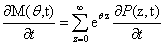
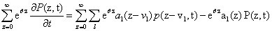
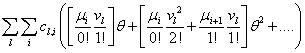
Since we would like to talk about moments of the CME rather than probabilities, our first priority is to write this equation in terms of M, rather than in terms of P. We multiply both sides by e^θz and sum over all possible values of z:

that taking into account the previous definitions results

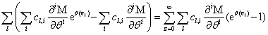
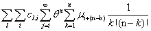
Now, we can take the second definition of and expand into its Taylor series. Notice that the summation now begins at j=i. When j < i, the index will be out of bounds and not correspond to any physical state

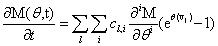
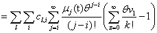
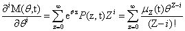
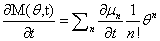
Remember that the initial goal was to isolate the coefficients of θⁿ in order to obtain the nth moments:

Our next step will be isolate just the coefficients of θ in order to achieve a form in which we are creating ODE’s of μ rather than M (θ,t). Since

We will have to multiply both sides by n! in order to isolate μ. Thus, it finally results

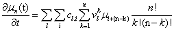
Closures

is easy to note from the previous expression [10] that the equation that governs the time evolution of the moments up to a certain order implies, in general, higher order moments, and then, before solving all them, higher order moments must be written as a combination of those involved in the considered time evolution equations. These relations have in most of cases an approximate character and are known as closure relations [12,15]. Before describing the technique that we are following for defining such closures for a given system, we introduce some notation.

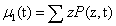
When considering multicomponent systems involving D components, the state becomes a vector Z^T = (Z₁,Z₂,……,Z_D) as previously discussed. Now the first moment also becomes a vector μ₁ of size D, defined by

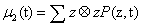
The second order moment μ₂ results a D×D matrix

μ₃ a third order tensor

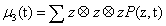
and so on. These expressions involve much symmetry e.g., μ₂ (i,j) = μ₂ (j,i)

In what follows and without loss of generality, we consider reactions involving linear propensities. Thus, when considering the equations governing the time evolution of the first two moments μ₁(t) and μ₂(t) the third order moment μ₃(t) remains in these equations, and it need to be expressed from both lower moments.

The simplest closure writes:

Where

and

Thus, the third order closure relation [16] involves 6 coefficients to be determined. For this purpose, and for a given system, we solve the CME by using the PGD in order to circumvent the curse of dimensionality and then evaluate the third order moment according to Equation (11) and then we choose the alpha parameters in Hegland et al. [16] to provide the best fitting (in a least squares sense).

As soon as the alpha parameters are empirically fitted, the CME is substituted by the two ordinary differential equations governing the time evolution of μ₁(t) and μ₂(t), when considering the solution of the same systems for any other initial condition or slightly different kinetic rates.

First, we consider the so-called Lotka model. This model consists of:

Where the number of molecules of species A and B are enforced to be constant. We consider the two simulation cases:

Case 1: At the initial time t = 0, the state of the systems consists of = (120,50), the reaction rates being λ1 = 1, λ 2 = 0:012 and λ3 = 1.

First, we solve the CME with the Case 1 conditions. The probability distribution function at 6 different times is depicted in Figure 1.

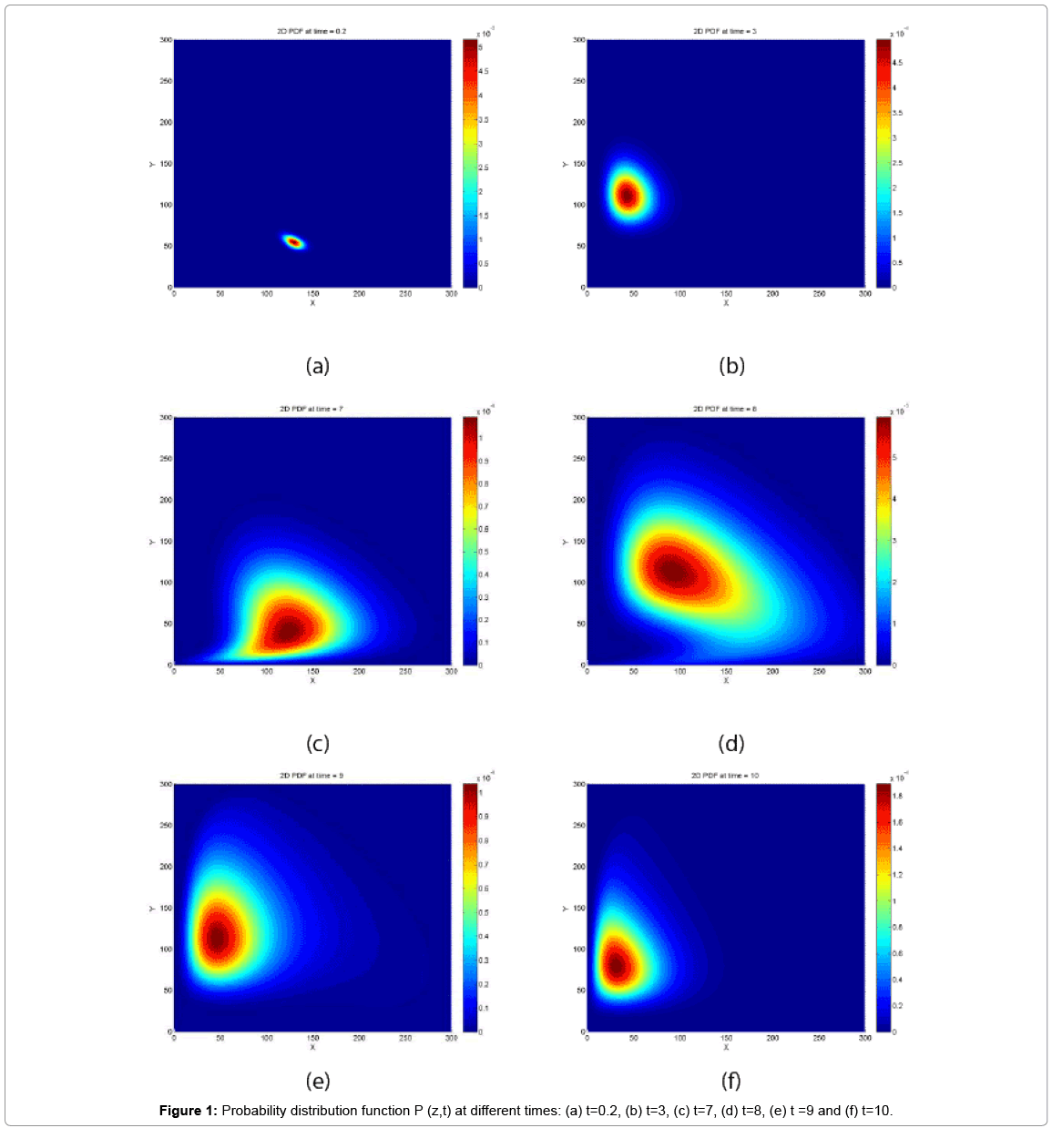
Figure 1: Probability distribution function P (z,t) at different times: (a) t=0.2, (b) t=3, (c) t=7, (d) t=8, (e) t =9 and (f) t=10.

Now from the pdf and t = [0,10], we compute the three first moments μ₁(t), μ₂(t), and μ₃(t), respectively from Equations (9-11) that will be considered as reference moment solutions. The parameters alpha involved in the empirical closure relation [16] are then determined. In the present case, and taking into account the symmetries, μ₁, is of size two, μ₂, has three independent components and μ₃, four. Figure 2 shows the different independent components of μ₁, and μ₂. Figure 3 compares the reference third moment with the one fitted with the empirical closure relation, from which we can conclude that both are in perfect agreement.

Figure 2: Time evolution of the components of μ1 (left) and μ2 (right).

Figure 3: Time evolution of the third order moment μ3(t): reference components (continuous line) versus closure-based approximation (broken line).

Now, by integrating in time the equations governing the time evolution of the components of μ₁, and μ₂, using the just identified empirical closure relation, we obtained the curves depicted in Figure 4 that are very close to those obtained from the probability distribution function that were depicted in Figure 2.

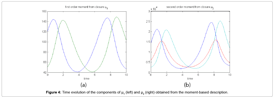
Figure 4: Time evolution of the components of μ₁ (left) and μ₂ (right) obtained from the moment-based description.

Now, with the closure relation obtained from the analysis of Case 1 we are addressing Case 2 without modifying the closure relation. For that purpose the equations governing the time evolution of the different components of μ₁, and μ₂ are integrated in time by considering the closure relation fitted in Case 1. In order to check the accuracy of those solutions we solve again the CME and compute the reference moments from the resulting probability distribution function. Figure 5 compares the moment-based and the pdf-based moments. Even if non negligeable deviations in the second order moment are noticed at the final time, results are qualitatively quite good.

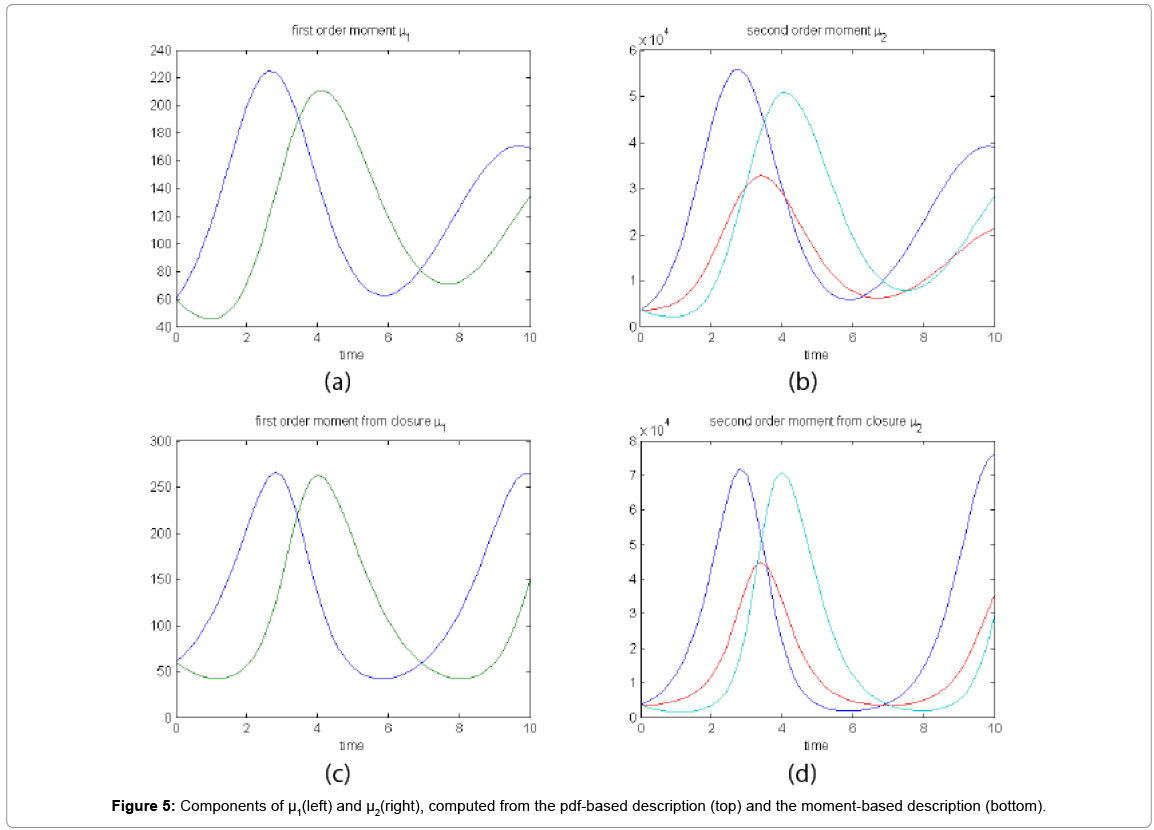
Figure 5: Components of μ₁(left) and μ₂(right), computed from the pdf-based description (top) and the moment-based description (bottom).

Exclusive switch 5D model

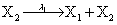
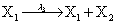
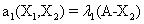
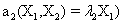
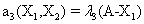
We consider a gene regulatory network called exclusive switch. It describes the dynamics of two genes with an overlapping promoter region, and the corresponding proteins X₁ and X₂. Both X₁ and X₂ are produced if no transcription factor is bound to the promoter region.

However if a molecule of type X₁ (X₂) is bound to the promotor then it inhibits the expression of the other protein i.e., molecules of type X₂ (X₁) cannot be produced. Only one molecule can be bound to the promotor region at a time which gives three possibilities for the state of the promoter region (free, X₁ bound, X₂ bound). The model is infinite in two dimensions (X₁ and X₂) and the reactions are given by:

where (λ₁,λ₂,…..λ₁₀) = (2,5,0.005,0.005,0.005,0.002,0.02,0.02,2,5). The initial conditions are such that only one DNA molecule is present in the system while the molecular counts for the rest of the species are zero.

First, we solve the CME. The probability distribution function at 6 different times is depicted in Figure 6.

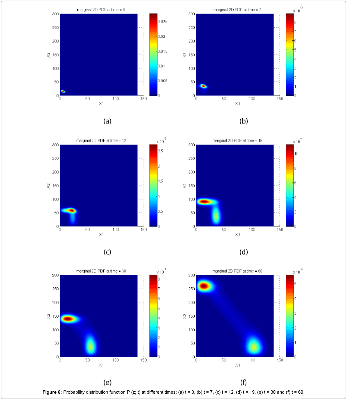
Figure 6: Probability distribution function P (z; t) at different times: (a) t = 3, (b) t = 7, (c) t = 12, (d) t = 19, (e) t = 30 and (f) t = 60.

Now from the pdf P(z,t) = (#X₁,….#X₂) and t = [0,60], we compute the three first moments μ₁(t), μ₂(t), and μ₃(t), respectively from Equations (9-11) that will be considered as reference moment solutions. The parameters alpha involved in the empirical closure relation [16] are then determined. Figure 7 shows the different independent components of μ₁ and μ₂. Figure 8 depicts the fitted third moment that makes use of the empirical closure relation.

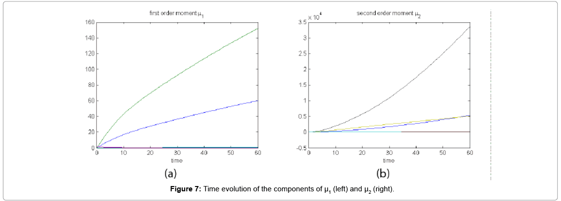
Figure 7: Time evolution of the components of μ₁ (left) and μ₂ (right).

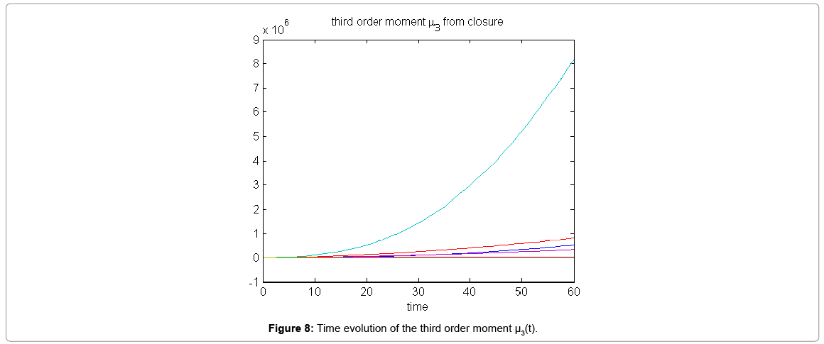
Figure 8: Time evolution of the third order moment μ₃(t).

With the closure relation just identified we are addressing a new scenario consisting of a different initial condition = (50,100,0,0,1) that produces at time t=10 the pdf depicted in Figure 9. Now, the equations governing the time evolution of the different components of μ₁ and μ₂ are integrated in time by considering the closure relation just identified fitted. In order to check the accuracy of those solutions we solve again the CME and compute the reference moments from the resulting probability distribution function. Figure 10 compares the moment-based and the pdf-based moments, proving that the moment approach based on the use of an empirical closure produces a quite reasonable agreement.

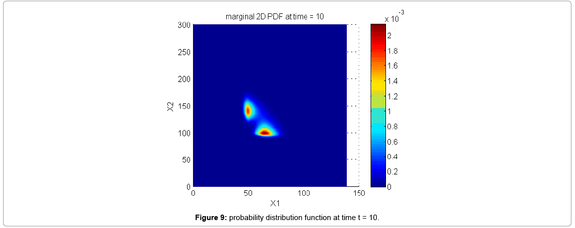
Figure 9: probability distribution function at time t = 10.

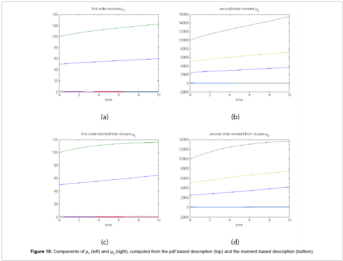
Figure 10: Components of μ₁ (left) and μ₂ (right), computed from the pdf based description (top) and the moment-based description (bottom).

The toggle

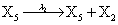
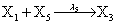
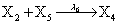
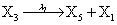
Mutually repressing gene pair, or gene toggle, can be found in biological systems as discussed in Hegland et al. [16]. As in their example, here we focus on protein dynamics, and more particularly in the toggle-switch network. The reactions consist of:

and the following polynomial properties are considered:

Now, we consider the initial condition as well as the parameters λ₁=1, λ₂=5, λ₃=1 and λ₄=10, and solve the associated chemical master equation for calculating the joint probability distribution function P (z,t). Now from the pdf P(z,t), z^T = (#X₁, #X₂) and t = [0,1], we compute the three first moments μ₁(t), μ₂(t), and μ₃(t) respectively from Equations (9-11) that will be considered as reference moment solutions. The parameters alpha involved in the empirical closure relation [16] are then determined. Figures 11- 13 compare respectively the different independent components of μ₁, μ₂, and μ₃ calculated from chemical master equation solution and from the closure-based description. A very good agreement can be noticed.

Figure 11: Time evolution of the components of μ₁ calculated from the CME solution (left) and from the closure-based description (right).

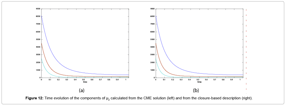
Figure 12: Time evolution of the components of μ₂ calculated from the CME solution (left) and from the closure-based description (right).

Figure 13: Time evolution of the components of μ₃ calculated from the CME solution (left) and from the closure-based description (right).

With the closure relation just identified we are addressing a new scenario consisting of a different initial condition =(1,1). Now, the equations governing the time evolution of the different components of μ₁ and μ₂ are integrated in time by considering the closure relation just identified fitted. The third moment is calculated from the fitted closure from the first two moments. In order to check the accuracy of those solutions we solve again the CME and compute the reference moments from the resulting probability distribution function. Figures 14-16 compare respectively the different independent components of of μ₁, μ₂, and μ₃ calculated from chemical master equation solution and from the closure-based description. Again a very good agreement can be noticed.

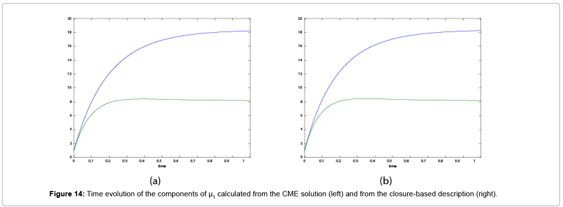
Figure 14: Time evolution of the components of μ₁ calculated from the CME solution (left) and from the closure-based description (right).

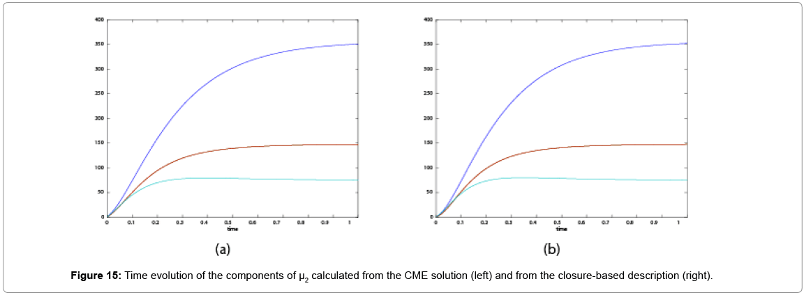
Figure 15: Time evolution of the components of μ₂ calculated from the CME solution (left) and from the closure-based description (right).

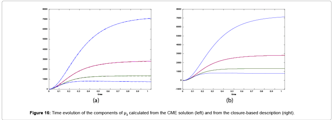
Figure 16: Time evolution of the components of μ₃ calculated from the CME solution (left) and from the closure-based description (right).

In this work we revisited the modeling of regulatory networks described within the chemical master equation framework. Deterministic solutions of the CME were performed by using the separated representation involved in the PGD, allowing circumventing the so-called curse of dimensionality. In order to improve the computational efficiency a moment-based description is derived, however such description involves higher order moments that must be described from the ones of lower order. In that sense we proposed a simplest closure relation, of empirical nature, that can be fitted numerically from the probability distribution function, the last coming from the PGD solution of the CME. As soon as the closure relation is fitted, it can be used for solving similar problems to the one that served to identify the closure relation.