Journal of Climatology & Weather Forecasting

If there were a way to know what the weather pattern would look like in the next few hours, days, weeks, and months, then weather forecasting accuracy would get a big boost. Cycling weather patterns have been studied for more than 70 years now, and this paper is an evolution of research that has been taking place since at least the 1940s. The Cycling Pattern Hypothesis, introduced in this study, provides a solution to many short and long-range weather forecast problems that exist in meteorology today. Imagine having the ability to know that the western United States drought was likely to be wiped out in the 2016-2017 weather patterns as early as October or November of that early season, which will be showcased in this paper. Jerome Namais (1910-1997) was an “influential meteorological researcher who pioneered extended weather forecasts in the United States New York Times Article: (http://www.nytimes.com/1997/02/12/us/jeromenamias-weather-forecasat-expert-dies-at-86.html). Namias wrote more than 200 papers and published a few books, including “Extended Forecasting by Mean Circulation Methods” in 1947. In 1950, Namias advanced his work and published a paper called “The Index Cycle” [1].

In addition, he proposed these questions in addressing long-range weather forecasting in his summary 1 Why during each year is there a tendency for the occurrence of at least one index cycle lasting a few weeks? 2 Why do these cycles vary from one year to the next? Namais summarizes “Because for reasons unknown, the quasi permanent anchor troughs and ridges are fixed in different regions in different years”. 28 years later, Namais had a paper published titled, “Multiple Causes of the North American abnormal winter 1976-1977” [2]. He suggested that there is enough information, evidence in the fall months to make a long-range prediction for that next winter season, “The signals of the oncoming winter’s patterns were clear enough by November to permit a reasonably successful long-range forecast”. There were three important points that Namais made in his research that are discussed in the Cycling Pattern Hypotheses, hereafter referred to as the CPH.

Was Jerome Namais onto something of extreme importance for the science of meteorology? Why is it taking so long to add this weather forecasting technology to the scientific community? The biggest reason may be that, until now, this technique was more observational and intuition, as was the likely technique used by Namais before computer technology arrived. This upcoming study, independently discovered by the authors 30-years ago, is introducing an evolution of what was potentially discovered over 70 years ago by Namais, that there is organization to the chaos of the river of air flowing above the surface in the troposphere; a cycling pattern that repeats. It will be presented and shown that the qualitative work can now be quantified with accurate results.

The science of weather forecasting has evolved tremendously over the past few decades. With all of the advances in the field of meteorology, it is widely believed that there is a 15-day limit in forecast skill. This has been cited in numerous papers [3]. Today, some forecasts delivered by TV meteorologists go out seven to 12 days with a limited amount of accuracy, while forecasts with three days to a week of leadtime barely had any skill a couple of decades ago. Indeed, the Weather Prediction Center (WPC) three-day quantitative precipitation forecasts are as accurate today as one-day forecasts were around 20 years ago [4]. The same article also notes that MOS mean absolute errors for seven-day temperature forecasts in 2012 were the same as they were for a three-day forecast in the early 1980s (averaged over the CONUS).

In addition to increased accuracy in weather forecasting in the one to seven day range, there has been increased emphasis on improving seasonal forecasts over the past couple of decades. For example, Colucci and Baumhefner examined the accuracy of 30-day 500-hPa height anomaly forecasts [5]. The study determined that the accuracy of the 30-day forecasts was somewhat dependent on initial conditions. More recently, Gershunov et al. examined the year-to-year variability of atmospheric river events affecting the west coast of North America, citing several factors that influence their intensity [6]. Gensini analyzed the predictability of tornado outbreaks two to three weeks in advance using a combination of factors, notably the Global Wind Oscillation [6].

While Gensini [6] focused on tornado outbreaks, this study aims to display a cycling pattern hypothesis that allows the operational forecaster to predict not only tornado outbreaks, but also other potential significant weather events weeks to months in advance. This CPH technology may very well help businesses and consumers plan and prepare with confidence.

There appears to be evidence cyclicality plays a significant role in the weather we experience here on earth. There are many possible causes of this cyclicality: sea surface temperature anomalies, the tilt of the earth’s axis, temperature anomalies of the air masses, and a combination of other forcing mechanisms still being identified. Cycling patterns have been studied over the past few decades.

The Madden-Julian Oscillation (MJO), which has been accepted in the scientific community, shows that there is a cycling pattern of incoming and outgoing long-wave radiation, which is showcased by convective complexes within the tropical regions of the earth. In 1971, Roland Madden and Paul Julian stumbled upon a 40-50 day oscillation when analyzing zonal wind anomalies in the tropical Pacific [7]. The MJO, also referred to as the 30-60 day oscillation, turns out to be the main intra-annual fluctuation that explains weather variations in the tropics. From Matthews [8], “accurate forecasting of this variability will benefit people living in the tropical regions, and also over the rest of the Earth due to remote ‘teleconnections’ between the weather in the tropics and the weather elsewhere around the globe.” It is accepted that there is a cycling pattern within the tropics. Why wouldn’t the pattern also be cycling regularly within the westerly belt?

In addition to the MJO, other oscillations have been studied for decades and are currently being analyzed today, such as the Arctic Oscillation (AO), North Atlantic Oscillation (NAO), Pacific Decadal Oscillation (PDO), and many more. More details about these teleconnections can be found on the NOAA CPC website. These teleconnections have shown some cyclicality as well, but with little known predictability. The weather forecaster that uses a growing understanding of all of these parameters, combined with knowledge of what is being presenting in the CPH, will be able to develop some skill in forecasting the weather beyond 15 days.

While Namais may have discovered something rather significant in the 1940s and 1950s, this paper is a proposed advancement of Namais’ work.

The cycling pattern hypothesis (CPH) there are three main aspects to this new hypothesis

• A unique weather pattern within the troposphere, evolves and develops every year in the early fall, roughly between around 1 October and 30 November.

• Long-term long-wave troughs and ridges that become established, called quasi-permanent anchor troughs and ridges by Namais. These features develop over the Northern Hemisphere every fall and are in different locations each year. These broad synoptic scale features, seen in the 500-hPa charts, are where storm systems reach their peak strength, near the anchor troughs, and they are most often at their weakest near the anchor ridges, and line up in different positions in each cycling pattern year. The smaller features, the short wave troughs, vorticity maximums, etc. are influenced by how these anchor troughs and ridges set up each year. These smaller features have been found to also be unique to that current years pattern and important factors to understand to help make accurate weather predictions for what is experienced at the surface.

• A cycle length evolves, becomes established by sometime in December each year, and then the cycle and pattern continue in a regular range through the rest of fall, winter, spring, and summer. In the 2016-2017 season the pattern was likely cycling in a 56 to 61 day range, centered on 58.5 days; i.e. if the first cycle is 58.5 days in length, then the second cycle will also be in that range and repeat. The entire cycle has been observed to repeat over and over again until the new pattern sets up the next October.

In studying and analyzing the weather patterns of the past few decades, it has been observed, by the authors of this paper, that a unique weather pattern sets up each fall, and this beginning of each year’s cycling pattern happens to coincide within just two weeks of the sun setting at the North Pole, about the time twilight ends and total darkness begins. There may be some connection to this, seemingly, coincidence, and it must be explored further in future studies. The weather pattern seems to begin each fall right around the same time the North Pole twilight ends.

The second aspect of the CPH is highly important for seasonal forecasting and so much more. Synoptic scale storm systems will reach peak strength and intensify into anchor troughs and weaken as they approach the anchor ridges. The locations near these long term longwave features will be affected by an above average number of storm systems near the anchor troughs, with a below average number of storm systems within a given season near the anchor ridges.

The third aspect of the CPH is perhaps of the utmost importance; a cycle length evolves, becomes established, and continues through the next summer. Once the cycle length is identified, if it is truly cycling with in the identified range in that year’s pattern, it can then be used to make rather specific weather forecasts down to a series of dates. If the forecaster has knowledge of the cycle length, then the part of the pattern that produces impacting storm systems can be predicted to return on cycle, and accurate weather predictions can be made. Broad seasonal forecasts for regions would be made with the potential of being accurate. For the forecast to be more specific, knowledge of how the 500-hPa flow will affect other significant levels down to the surface will need to be applied and tested. For example; if a city is affected by a long-term long-wave 500 hPa trough and thus experiences a large number of storm systems in October and November, one can confidently make a winter forecast for below average temperatures and above average precipitation. To identify specific high-impact storm systems in advance using only the 500hPa flow, the forecaster must carefully analyze each 500hPa wave that occurred during October/ November and figure out how each wave will affect other significant levels (e.g. 925, 850, and 700hPa) as well as the surface weather. Even though the 500-hPa pattern is likely cycling regularly, forecasts for surface weather with months of lead-time will sometimes be off by a few days or a few hundred miles.

Once a cycle is established, and then the entire cycle will then repeat over and over again until another unique pattern sets up the next fall. According to the CPH, the current year’s pattern fades, and the new pattern evolves and begins during a transition period near the end of September into early October. This limits the forecast accuracy to be from December through the next September and not beyond September, or around a 300-day limit in accuracy.

The CPH has been in use for the past 15-plus years with results being analyzed and tested. The cycle length, during the 2016-2017 seasons, became established in October and November as proposed by the CPH, and then continued through the rest of fall, winter, spring, and through the following summer in 2017. This study will show, both quantitatively and qualitatively, that a 56 to 61 day cycle became established by December in the 2016-2017 cycling pattern year. The cyclicality will be tested using a cycle length near the average of each range; i.e. 58.5-days in the 2016-2017 season. A cycling pattern year will be defined to be from 1 October of the current year to 30 September of the following year.

The meteorologist observing the cycling weather pattern will have the ability to pick out and identify the storm systems that will likely return in future cycles. This is done by analyzing upper level charts within the troposphere (mainly at the 500-hPa level) and then using the cycle length to project into the future, as was possibly a Namais technique in the 1940s and 1950s. The 500-hPa level was chosen because it is, on average, over 1000 meters above the highest mountains in the CONUS. Thus, topography at the surface will have minimal effects on the 500-hPa height field. The quantitative analysis will be presented as it uses this essential information, validating the likely cycle length and applying it to the forecast system. If the qualitative analysis matches the quantitative verification, then the model will have an increased chance of being accurate and the weather forecaster will gain confidence without even needing a computer model to help make a future forecast. The 500 hPa pattern over a few days can be projected into future cycles and then forecasts will be made for any location chosen in the Northern Hemisphere.

Over the past 15 years, the CPH has been documented (shown below) with cycle lengths identified by mid-December each year. Utilizing knowledge of this innovative forecast method, hundreds of forecasts have been made, many of them quite accurate, while other forecasts failed. What has also been observed is that the cycling pattern itself rarely ever fails; i.e. the pattern has been shown to always be cycling in the ranges identified. The inaccurate forecasts come from the weather forecaster that is attempting to use the CPH in making these weather predictions, and then the storm ends up arriving, but it may just miss the forecast verification site. Forecasting low-level jets and other features that will impact weather events must be considered. Having a strong understanding of how the flow is analyzed at the 500- hPa level can be used to forecast how features at other significant levels will line up, and this will increase the probability of a successful forecast. Examples of the CPH were found through qualitative analysis of the 500-hPa maps. Later in this paper, we will show the qualitative analysis from the 2016-2017 season, and quantitative validation from three CPH years. Here are the cycle lengths that were documented through observational analysis in recent years:

• 2002-2003: 35 to 40 days (37.5 day average)

• 2003-2004: 52 to 56 days (54 day average)

• 2004-2005: 73 to 77 days (75 day average)

• 2005-2006: 60 to 62 days (61 day average)

• 2006-2007: 42 to 48 days (45 day average)

• 2007-2008: 52 to 54 days (53 day average)

• 2008-2009: 50 to 53 days (51.5 day average)

• 2009-2010: 58 to 62 days (60 day average)

• 2010-2011: 50 to 52 days (51 day average)

• 2011-2012: 45 to 49 days (47 day average)

• 2012-2013: 50 to 57 days (53.5 day average)

• 2013-2014: 55 - 61 days (58 day average)

• 2014-2015: 43 to 50 days (46.5 day average)

• 2015-2016: 47 to 52 days (49.5 day average)

• 2016-2017: 56 to 61 days (58.5 day average)

During the past 30 years, a long-range forecasting system has been developed and having an understanding of the cycle length is essential when making weather forecasts based on this new hypothesis. We will scientifically examine this evolving system to establish the validity to this proposed methodology for weather prediction.

A cycling pattern index and correlation coefficient

To validate, what is found qualitatively through map-to-map comparisons, a quantitative analysis of the 500-hPa height fields for various locations has been completed. One metric that is being developed and tested to showcase the cycling of the 500-hPa heights are the Cycling Pattern Index (CPI), and another 500-hPa analysis, that has been named, the Eastern Pacific Blocking Index (EPBI). These are calculated using the following formulas:

• The Cycling Pattern Index (CPI) = (H5 – H5ave)/ 6 (Using Chicago, IL 500-hPa heights and averages at 12z each day

• The Eastern Pacific Blocking Index (EPBI) = (H5 – H5ave)/ 6 (Using Seattle, WA 500-hPa heights and averages at 12z each day

Each of these indexes is an analysis, where H5 represents the 1200 UTC 500-hPa height in decameters and H5ave represents the 30-year average hPa height for a particular location. Chicago, IL has been selected as the evaluated location, for the CPI, because it is frequently affected by the northern stream of the 500-hPa jet as storm systems track near-just north or just south of-this region. The EPBI is an analysis of the 500-hPa field at Seattle, WA. If the index is high near Seattle, then there is likely a blocking ridge near the west coast; thus the name Eastern Pacific Blocking Index. The equation divides by six to have the index end up in a range to look similar to the Arctic Oscillation and North Atlantic Oscillation indexes. Other locations have been studied with results quite similar to the ones we are presenting in this study. These other locations will be analyzed in future work of the cycling pattern verification.

Correlation coefficient r was calculated in comparing one cycle to the other cycles within that CPH year. More specifically in the 2016-2017 CPH year, 20-day and 30-day stretches were analyzed for potential cycle lengths from 50 to 65 days (one cycle length) apart.

This was done in order to see if there was a correlation in comparing cycles based on the qualitatively observed cycle length. In other words, the cycle can be found through qualitative map-to-map comparisons as shown in Figure 1 & Figure 2 (initial analysis of the 500-hPa height fields) from one cycle to the next. If there is truly a regular cycle length, that oscillates through the date ranges identified through the qualitative analysis, for almost an entire year (October through September), it should show up in the quantitative analysis through comparing cycles.

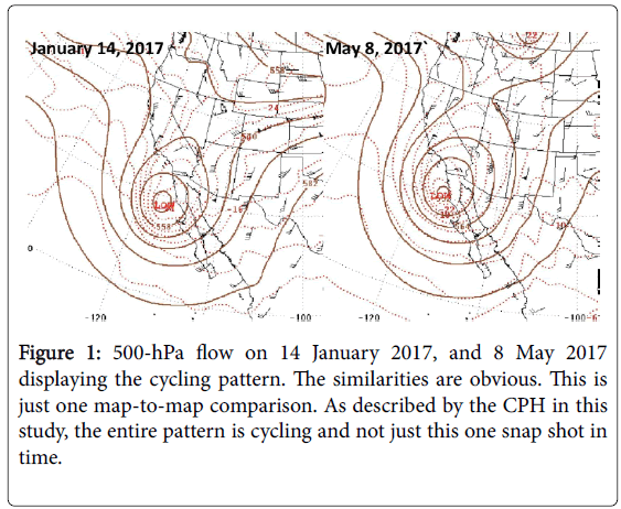
Figure 1: 500-hPa flow on 14 January 2017, and 8 May 2017 displaying the cycling pattern. The similarities are obvious. This is just one map-to-map comparison. As described by the CPH in this study, the entire pattern is cycling and not just this one snap shot in time.

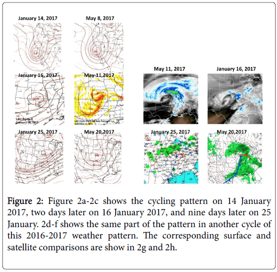
Figure 2: Figure 2a-2c shows the cycling pattern on 14 January 2017, two days later on 16 January 2017, and nine days later on 25 January. 2d-f shows the same part of the pattern in another cycle of this 2016-2017 weather pattern. The corresponding surface and satellite comparisons are show in 2g and 2h.

Over the past 15 years of analyzing these cycles and experiencing the cycling pattern in real time by meteorologists through observation and comparing actual 500-hPa verified analysis maps of the Northern Hemisphere, we would expect correlation coefficient r to be the highest value near the observed cycle length. We still do not expect r to approach 1 over the entire cycle, as the cycle length is constantly changing or oscillating between the observed 56 and 61 days in the 2016-2017 season.

In the smaller sample sizes within 20-30 day stretches, r is expected to approach 1 more often. Over the entire cycle length we consider r>=0.3 (weak correlation) to be a result that signals some degree of cycling in the 500-hPa height pattern. Correlation coefficient r was calculated for a full cycle length and the shorter periods where the patterns seemed to line up the best by qualitatively analyzing the 500- hPa charts.

Analysis from the two previous years has also been statistically analyzed with results rather clearly showing r -values, which validate the cycles found qualitatively. This analysis can be seen in Figures 3a-3c.

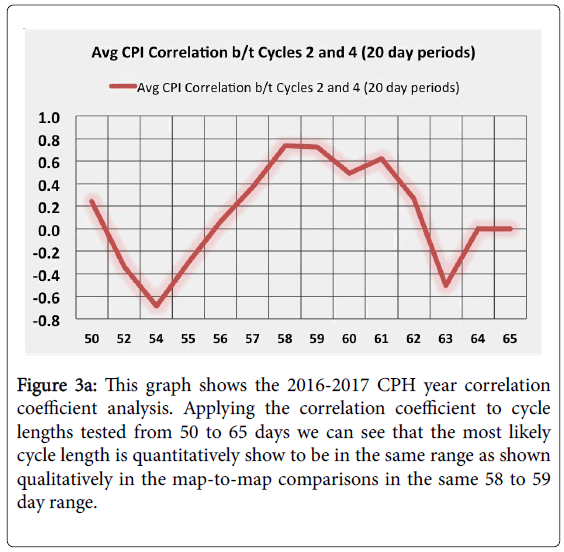
Figure 3a: This graph shows the 2016-2017 CPH year correlation coefficient analysis. Applying the correlation coefficient to cycle lengths tested from 50 to 65 days we can see that the most likely cycle length is quantitatively show to be in the same range as shown qualitatively in the map-to-map comparisons in the same 58 to 59 day range.

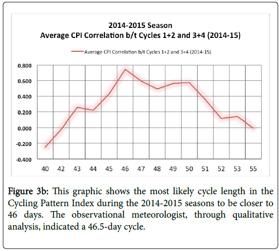
Figure 3b: This graphic shows the most likely cycle length in the Cycling Pattern Index during the 2014-2015 seasons to be closer to 46 days. The observational meteorologist, through qualitative analysis, indicated a 46.5-day cycle.

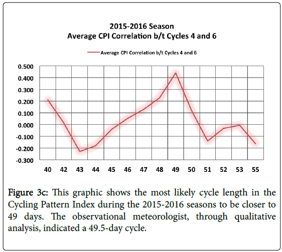
Figure 3c: This graphic shows the most likely cycle length in the Cycling Pattern Index during the 2015-2016 seasons to be closer to 49 days. The observational meteorologist, through qualitative analysis, indicated a 49.5-day cycle.

Experimental forecasts and statistical analysis

Most zip codes across the United States are being tested and studied with experimental month-long heating degree-day (HDD) forecasts issued one to nine months in advance. HDDs are a measure of temperatures for each location, a measurement designed to quantify the demand for energy needed to heat a home or office building. HDDs are directly related to temperatures, so using this parameter is a great way to measure locations forecast accuracy when comparing the average to what a model would forecast for each location.

65°F (18.3°C) is used as the baseline. An HDD is zero if the average temperature for that day is 65°F (18.3°C). If the average temperature is 30°F (-1.1°C) for that location, then the HDD would be 35°F (19.4°C).

We will be using degrees Fahrenheit for this paper, as this is the common use in the United States.

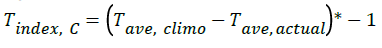
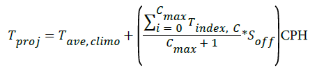
These forecasts for each zip code are using a CPH model that has been applied by taking what happened in previous cycles of the current year’s pattern, and projecting forward. After indexing each day within each previously occurring cycle since the cycle start date, each day’s temperature offsets were calculated. This was achieved by taking the daily average temperature T_ave,climo ([high + low]/2) and subtracting the actual recorded daily temperature T_ave,actual (again both high and low combined) and multiplying by negative one to preserve the sign for future summation. Here is the formula that was used:

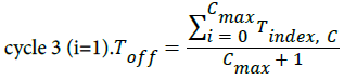
Then when projecting to a future date, each of that day’s cycle index temperature offsets were averaged (for both high and low combined). C_max represents the number of cycles (minus one) that were used to project forward in time. For example, if we want to use recorded data from cycles 2 and 3 to make a projection for cycle 4, then C_max would equal 1. In this case, we would have to calculate T_index,c ( C_max+ 1) times (twice in this example): once for cycle 2 (i=0) and then again for

To then project temperatures forward for the desired period of time, the day’s averages were added to the seasonally adjusted previously calculated offsets. The seasonal adjustment (S_off) was used to prevent seasonally impossible extreme temperature differentials from influencing temperature projections. T_ave,proj represents the daily average temperature for the projection date. T_proj represents the forecast daily average temperature for the projection date.

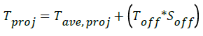
Combining the second and third formulas above, the projected temperature can be calculated as follows:

model forecasts were compared to HDD forecasts issued purely using climatology. Both qualitative and quantitative comparisons were made to verify the cycle length. Here are the three ways that we will measure the accuracy of our experimental forecasts.

• Comparing the average line forecast Climatology to the actual forecast line and verifying which forecast was closer to what actually happened at each location is the first way to measure accuracy.

• A second way to measure accuracy is by measuring the actual HDD monthly total to what was verified by the end of each month.

• A third way to measure accuracy would compare the CPH model to what is produced by any other method.

For the quantitative comparison, a t-test was carried out. The null hypothesis was that the CPH model forecasts were equal in accuracy to the Climatology forecasts. The alternative hypothesis was that the CPH model forecasts were more accurate than the Climatology forecasts. A significance level of alpha=0.05 was used to determine if the CPH model forecasts were significantly more accurate.

Results: Qualitative analysis of the cycling pattern

A meteorologist making weather forecasts uses a combination of art and science on a daily basis. Numerical weather prediction (NWP) models such as the Global Forecast System (GFS), European Model for Medium-Range Forecasting (ECMWF), and North American Mesoscale Model (NAM) are utilized to help make these forecasts. The CPH is a new technique wherein the forecaster uses knowledge of what has already happened within that year to have a good idea of when these NWP models are accurate, and when they are likely inaccurate.

The operational forecaster can go one step further, using previous cycles to “know” what the pattern will likely look like by analyzing 500-hPa maps from previous cycles. If the cycle length is known, the forecaster has insight into what the pattern will likely be in future cycles, and thus can make a prediction from a few hours to up to 300 days into the future. This “art” is used all of the time by the operational forecasters around the world. This process, if quantified, could add another data layer into current weather forecast models being used today to increase accuracy, or it could be a stand-alone model.

According to the CPH, the part of the cycling pattern that produced storm systems in October and November will likely return in December and January, the next cycle. It isn’t just one stretch of three to five days that produces a storm system that is repeating, but rather the entire weather pattern that is cycling and repeating regularly.

Once these repeating features are identified, the cycle length can be determined (typically in December) and confirmed in the following weeks and months. Once the cycle length is confirmed, the forecaster can use previous cycles and project forward to each day from January through the next September. If the pattern is indeed cycling regularly, then the weather forecasts made using this technique will have a good chance of verifying. A few examples are presented in this study.

The area of analysis is from the eastern Pacific, across North America, and into the western Atlantic, but it will be applied, in future studies, to any other location in and close to the westerly belt across the Northern Hemisphere. When one cycle is completed, 58.5-day average cycle in the 2016-2017 season, then the second cycle will begin and again last an average of 58.5 days. These cycles repeat until another unique pattern sets up the next fall. During the 2016-2017 CPH year, the cycle length was shown to be in the 56 to 61 day range, centered on 58.5 days. So, cycles 2-4 and so on will line up from cycle to cycle as the pattern continues into September. This will all then reset in October, as proposed by the CPH.

In Figure 1 the similarities in the pattern on 14 January 2017 and 8 May 2017 are quite obvious when looking at the upper lows near the Baja California coast south of San Diego, CA. The strengths and position of the 500-hPa low are almost identical. These dates are 114 days (2 cycles) apart. The meteorologist skilled in reading the cycle length of 56 to 61 days of the 2016-2017 pattern can look at January 14 and forecast that there will be a return of this pattern within one to three days of 8 May as shown in Figure 1. In this example, an accurate four-month forecast can be made.

If you do not know what the cycle length is, then the information from January is useless. But, if you do know that the pattern is cycling in the 56 to 61 day range, then the forecast would be made for this part of the pattern to return around May 8th, and that it would look similar to January. The cycle length must be applied in this forecast method. The organization to the chaos comes together with the understanding of the CPH.

The CPH is a description of the entire pattern, not just the two snap shots in time as shown in Figure 1. A couple of days after the 14 January 2017 and 8 May 2017 example and comparison, a storm emerged in the plains states and a major ice storm was forecast by many sources. In May, also several days later, a similar storm system developed, as shown in the sequence of maps shown in Figure 2. The pattern then continues to cycle regularly according to the CPH, and nine days later, there is another storm emerging over the plains in January and in May, right on “schedule” by applying this CPH system, a similar system also emerges. There are obvious seasonal differences as the energy in the flow is much stronger in late January than it is in late May.

Once this pattern sets up in January, the weather forecaster using this qualitative approach will have enough information to make forecasts for any location chosen within the westerly belt. These weather forecast predictions would be made in January, projected into future dates through the next September. The forecaster can make accurate forecasts for significant levels from the surface all the way through the troposphere solely based on the cyclicality of the 500hPa flow. This allows the weather forecaster to do two important things: one Make a CPH system forecast days to months into the future, and two “Know” when the operational NWP models used today are potentially accurate or off base, if they do not “fit” what happened in previous cycles.

So, in this example, again using Figure 1; if a model did not show a storm around that particular date, then the forecaster can “know” that the model is likely wrong. One of the models may show a 240-hour 500hPa height forecast that looks similar to that January 14 storm, valid on May 8th. The forecaster can then “know” that the model is likely making an accurate projection of the pattern.

A major challenge for the forecaster is having an understanding of seasonal differences in the strength within the 500-hPa flow. The jet stream strength (measured by wind speeds) can be just as strong in May as it is in January. The seasonal differences can be seen in the amount of energy in the flow aloft, which will be stronger in January and February than it will be in May.

Even with some rather significant differences in this energy from season to season, the same pattern will likely cycle back through according to the CPH. As similar as the maps look in Figures 2a and 2b above, the overall pattern had major differences in strength. Predominant features, however, will often have similar strength as shown in this example. A forecast using what already happened in January can be made for this entire stretch in May, and in other cycles when applying the CPH forecast system.

Imagine the impact on the art of weather forecasting if the meteorologist could have in their forecasting arsenal the ability to “know” what the 500hPa height pattern will likely look like days, weeks, or even months before a major impacting weather event or disaster will occur. This is entirely possible and knowledge of the cycling pattern is being tested every day, and has been tested over the past two decades in operational forecasting.

These are examples showing organization in the chaos in the river of air flowing overhead impacting the surface of the earth, and the pattern is likely cycling regularly across the Northern Hemisphere, as described by the CPH. Any model developed using this technology could potentially be used both scientifically and in the business risk management environments. The benefits will likely be huge, both for the safety of people worldwide and financially.

Results: Quantitatively analyzing, validating, and verifying the cycling pattern hypothesis

Figure 4 shows the CPI (discussed in section 2a) values for cycles 1 through 5 overlaid on top of each other. Assuming the cycle length is close to 59 days, this cycle length was used to showcase the pattern. Chicago was the chosen location to measure the cycling weather pattern, the CPI for reasons discussed in section 2a. Many other zip codes have been tested showing similar results. A dip in the pattern showcases a storm moving by, and a rise in the pattern showcases likely higher heights and a lack of storm systems.

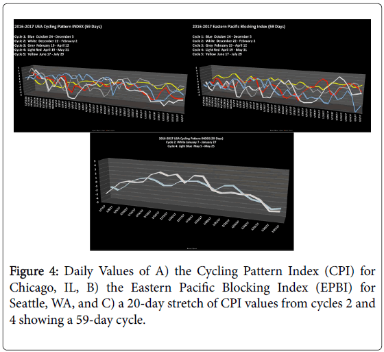
Figure 4: Daily Values of A) the Cycling Pattern Index (CPI) for Chicago, IL, B) the Eastern Pacific Blocking Index (EPBI) for Seattle, WA, and C) a 20-day stretch of CPI values from cycles 2 and 4 showing a 59-day cycle.

Figure 4 shows what is called the Eastern Pacific Blocking Index (EPBI). Seattle, WA was used for this index as, if the heights are high— shown with a positive index—there is an increased likelihood of blocking near the west coast and California will most likely be dry due to the likely jet stream flowing far to the north, thus blocking storm systems.

In the qualitative analysis, the 500-hPa during the 2016-2017 cycling pattern was observed to be in the 56 to 61 day range centered around 58.5 days. This analysis was done and validated with observations of the actual 500-hPa flow that had already occurred in the first two cycles of the pattern. Cycle 1 can be argued to begin around the end of the first week of October, with cycle 2 beginning 56 to 61 days later around the first week of December, cycle 3 likely beginning in early February, and so on. The cycle length evolves each year in the fall with a new cycle length setting up each year between October 1st and December 15th.

Figure 4 shows the 56 to 61 day cycle varying by a day or two from cycle to cycle. A cursory subjective analysis shows that the CPI values of cycles 1 and 2 match up very well-with the exception of a large dip in cycle 2-near the end of the first half of each cycle. Correlation coefficients of CPI Indices between cycles 1 and 2 were calculated for periods of different lengths. For example, in a 59-day cycle the period of 1 November-30 November in cycle 1 would correspond to 29 December-27 January in cycle 2. We were able to identify a 30-day period with a moderate correlation r=0.52. The dates with r=0.52 were 13 November-13 December and 11 January-10 February (Figure 4).

It makes sense that while we see a moderate correlation for the 20-30 day stretches of cycles 1 and 2, we did not see r-approaching 1 for any of the date ranges that were examined. This is likely because the CPI length fluctuates slightly; it does not always have a cycle length of exactly 57, 58, or 59 days. This means that today the 500-hPa heights may resemble what happened 57 days ago, while in a week they may resemble what happened 61 days ago. In this 2016-2017 example, the cycle length ranges from 56 to 61 days, but over the entire year’s pattern the cycle length will likely still fall within the average length of 58 to 59 days. The correlation coefficient (r) calculations are based on how day one correlates with day 60, day two correlates with day 61, and so on; therefore, r will be very sensitive to these slight fluctuations in cycle length. In essence, having a moderate correlation of the CPI and EPBI in a statistical sense when assuming exactly a 59-day cycle is strong evidence that there is indeed an organization to the chaos in the atmosphere.

A calculation was conducted of correlation coefficients of the CPI values for the entire 59-day stretch in cycles 2 (22 December-19 February) and 4 (19 April-15 June). These two cycles were chosen because they seemed to line up best when doing the qualitative analysis (for example, see Figure 1 and Figure 2). A correlation coefficient of r =0.51 was calculated between the entirety of the CPI values of cycles 2 and 4. Computing correlation coefficients of CPI values for similar 58- day periods also gave us values of around r=0.50. Lastly, we calculated the correlation of various 20- to 30-day stretches of CPI values between cycles 2 and 4 (the two cycles that lined up best qualitatively). In our observations (Figure 4) we can clearly show how cycle 2 matches up with cycle 4 quite often. In analyzing various 20 to 30 day stretches we can see r-approaching 1 in the 57.5 to 58.5 day ranges. This tells us two things: 1) our qualitative analysis showing that cycles 2 and 4 matched up the strongest was validated and 2) we achieved a strong correlation for the selected date ranges, which is very strong evidence of cyclicality of the 500-hPa height pattern.

Testing of a forecast model using the CPH

This technique of utilizing knowledge of the cycling pattern, as proposed by the CPH, may alone provide enough information to make accurate season-long forecasts. Over the past few years, a weather forecast model has been developed, that has been tested on HDD forecasts for various locations around the United States. This forecast model uses the temperatures and precipitation recorded at the official ASOS/AWOS stations approved by the National Weather Service. The model takes what has happened in the first cycle and projects forward with a forecast output for various temperature and precipitation parameters and has also been tested by blending cycles as the pattern moves into a third, fourth, and fifth cycle. This is a first attempt at using what has happened in a CPH year and projecting into future cycles. It should be emphasized that this model will evolve over the years and we recommend it to be tested and improved. In the model, it is assumed that the surface temperature patterns cycle much like the 500-hPa height patterns. Of course, the cyclicality of the surface temperature patterns may not be as pronounced as it is for 500hPa heights. However, this is an attempt to make a surface forecast based on our knowledge that the 500hPa height pattern is cycling.

Initial statistical analysis, presented in this paper, demonstrates statistical reliability and validity for this cycling weather pattern model. Here are some examples from forecasts made with 2-month lead-time using the 2016-2017 cycling pattern years’ 59-day average cycle length: The result for the month of February 2017 at the Cadillac, MI zip code is shown in Figure 5. The blue line shows climatology, or average HDD values. The orange line is the model projection, and the green line is what actually happened for this zip code. In this example, 1184 HDD is the historical average during February. The CPH model projected 1075 HDD, while 944 were observed. This was a warmer than average month in Cadillac, MI, and the CPH model predicted a warmer month, which was more accurate than climatology.

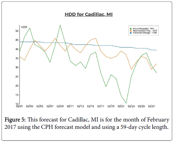
Figure 5: This forecast for Cadillac, MI is for the month of February 2017 using the CPH forecast model and using a 59-day cycle length.

It can be clearly seen in these two examples that the weather pattern is likely cycling at close to 59 days by comparing the green verification line to the orange forecast line. The model outperformed the average for February by 76 HDDs in Geneva, NY, as shown in Figure 6. In each of these two examples, this model outperforms climatology. In testing 100 other zip codes around the United States, two per state, this model outperforms climatology close to 75 percent of the time. These forecasts with 30-day lead-time are very valuable to many industries that depend on temperature, such as propane, natural gas, and agriculture (Figure 6).

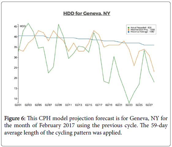
Figure 6: This CPH model projection forecast is for Geneva, NY for the month of February 2017 using the previous cycle. The 59-day average length of the cycling pattern was applied.

A t-test was conducted to show whether the model HDD forecasts outperformed climatology at a statistically significant level. The t-test between this model and climatology HDD forecasts yielded impressive results (Jan/Feb forecasts for the 100 zip comes). The p value was between 0.10 and 0.15 in favor of the CPH model. While not significant at the alpha=0.05 level, this is still evidence that there is a benefit to using the CPH, as the probability of the CPH model HDD forecasts (>1 month lead-time) being more accurate than climatology by chance is between 10 and 15 percent. This shows great promise in the application of this model to predicting weather elements at the surface over a month in advance based on the CPH at 500-hPa. We must keep in mind that this model is still evolving and there will be future advances that must be added and considered as we learn more about this long-range weather forecast system.

Applying the CPH: Predicting the ending of the Western United States drought during the extremely wet 2016-2017 winter season

In the 2015-2016 season the strongest El Niño ever recorded was developing and weather forecasts came out for drought-ending rains in California. The next winter a weak La Niña was developing and weather forecasts came out for a worsening of the western drought. The exact opposite happened in each of these El Niño/La Niña forecasts, as there was likely a stronger influence that must be considered, that could have helped prevent these forecast failures. The weather forecaster, applying the CPH forecast system proposed in this study, would likely have made much more accurate predictions. The forecast system emphasizing the CPH is shown to be a much better indicator of what will happen at the surface than the El Niño Southern Oscillation (ENSO). In a very broad sense, this is because the 500-hPa height field is more directly related to surface weather than ocean temperatures in the Tropical Pacific. With ENSO based forecasts the sea surface temperature anomalies are used to project broad weather patterns, so this method is sort of doing it the other way around.

• In the 2015-2016 drought-continuing year in California, there were many forecasts for way above average rainfall in California due to historic analysis of what happens with El Niño. One of the strongest El Niño’s developed during the fall of 2015 and instead of the forecast ending of the drought by many sources, California’s drought continued to expand.

• In the winter of 2016-2017, forecasts came out for a continuation of the major western drought due to the developing weak La Niña. What happened? The drought got wiped out as storm systems repeatedly blasted through California and the western United States, which was not forecast accurately by just using an understanding of the weak La Niña.

Teng and Branstator stated that a wave pattern is a global dynamic system that sometimes makes droughts or floods in California more likely to occur. The study also concluded that as we learn more, this might eventually open a new window to long-term predictability [1].

It is also discussed in Teng and Branstator that the finding is part of an emerging body of research into the wave pattern that holds the promise of better understanding seasonal weather patterns in California and elsewhere [1]. Another new paper examines the powerful wave pattern in more depth, analyzing the physical processes that help lead to its formation as well as its seasonal variations and how it varies in strength and location [8]. Again, Namias may have been stumbling across this technology over 70 years ago.

Through the understanding of the CPH, the problem presented by Branstator and Teng likely is answered. Let’s take a look at what happened in the Lake Tahoe region over the Sierra Nevada mountain range during the 2016-2017 cycling weather pattern. South Lake Tahoe precipitation in the 2016-2017 season:

• 14 to 17 October: 61 cm (2 ft) of snow above 8,000 feet and 12.75 cm (5.02 in) of liquid at lake level.

• 10 to 16 December: Over 152 cm (5 ft) of snow fell above (maybe need to convert this) 7,000 feet and 11.6 cm (4.58) inches liquid at lake level (57 to 60 days after the first big event, or an average 58.5 day cycle).

• 5 to 10 February: Close to 244 cm (8 ft) of snow reported above 7,000 feet with 19.7 cm (7.78 in) liquid at lake level (117 days after that first big precipitation event or a 58.5 day average cycle).

• 6 to 13 April: Close to 91 cm (3 ft) of snow was reported above 7,000 feet with 6.2 cm (2.46 in) liquid at lake level (174 to 178 days after the first big event in October or a 58-59 day cycle).

The wet season ends in late April over California, but even in June, in what was likely the fifth cycle of the 2016-2017 pattern, it snowed over the higher elevations around Lake Tahoe. 50 cm (19.84 in) or 43% of the seasonal precipitation total of 116 cm (45.67 in) fell when the storm systems, as described above, seemingly returned on schedule, while another 65.6 cm (25.83 in) fell in 54 of the other 186 days within the pattern, officially recorded at South Lake Tahoe, CA. These other wet storm systems, which also happened during the entire wet season, were a result of being close enough to one of the storm producing long term long-wave troughs as proposed in the second aspect of the CPH. The long-term long-wave positions set up to allow for the potential atmospheric river events and other storm systems to aide in ending the drought.

The weather pattern, through analysis of the 500-hPa height fields, in the first cycle can be projected to return in future cycles of the pattern. As proposed by this CPH it is the entire pattern that is cycling, not just a day here and a day there. These few map comparison examples can be shown across the entire cycle, not just one date, as it may seem. Figures 7a-7c show the 500-hPa charts for the first three cold season cycles, just one example of the cycling pattern that produced high precipitation set-ups over the western United States. These maps are from October 14th in cycle 1, December 11th in cycle 2, and February 7th in cycle 3.

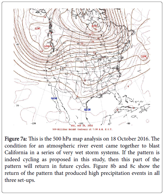
Figure 7a: This is the 500 hPa map analysis on 18 October 2016. The condition for an atmospheric river event came together to blast California in a series of very wet storm systems. If the pattern is indeed cycling as proposed in this study, then this part of the pattern will return in future cycles. Figure 8b and 8c show the return of the pattern that produced high precipitation events in all three set-ups.

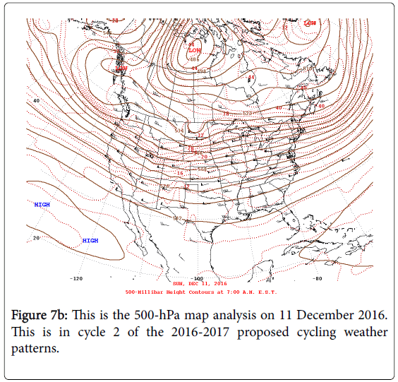
Figure 7b: This is the 500-hPa map analysis on 11 December 2016. This is in cycle 2 of the 2016-2017 proposed cycling weather patterns.

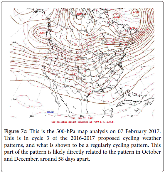
Figure 7c: This is the 500-hPa map analysis on 07 February 2017. This is in cycle 3 of the 2016-2017 proposed cycling weather patterns, and what is shown to be a regularly cycling pattern. This part of the pattern is likely directly related to the pattern in October and December, around 58 days apart.

These dates are exactly 58 days apart just as the excessive precipitation events were evolving over California. Again, let us stress that the entire pattern is cycling and not just the dates we are showcasing. So, the days leading up to the maps in Figure 7 and the days to weeks and months after the dates shown are also going to line up (Figures 7a-7c).

Figure 8 shows the HDD forecast and verification for South Lake Tahoe, CA. Climatology outperformed the model in this example, but the 59-day cycle can be seen by analyzing what happened from day to day compared to what was forecast by the CPH model. The test of the model shows the cycling pattern well, even though it may appear to be inaccurate on the HDD verification. The applied 59-day cycle length is quite visible, and the 58 to 59 day cycle can be shown in just about any zip code tested, which shows the likely organization to the chaos in the river of air above us.

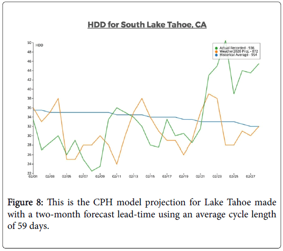
Figure 8: This is the CPH model projection for Lake Tahoe made with a two-month forecast lead-time using an average cycle length of 59 days.

A forecast for the end to the western drought could be made as early as October, certainly by December, emphasizing this proposed forecast system, knowledge of the cycling pattern, and other potential influences. The fact that a huge precipitation event occurred as early as October is important, but what caused it to happen is what is essential.

This CPH forecast system is being applied to predict these seasonal outlooks, but also cold outbreaks, heat waves, droughts, severe weather, and weather forecasts for every zip code in the United States with accurate results. Risks of severe weather can be predicted weeks to months in advance with knowledge of the weather pattern that already produced severe weather in previous cycles as well. Examples of dozens of these forecasts can be found in the weather blogs at KSHB.com and Weather2020.com [9,10].

There is likely something much bigger going on in the river of air above us. When diving deeper into this new hypothesis, the CPH, it seem rather obvious that there is an organization to what may seem like atmospheric chaos. Showing that there is regularity to cycling weather pattern, and one primary cycle, will provide the operational forecaster with great insight into what will likely be experienced at the surface. On the broad synoptic scale, it is being shown that the patterns are predictable and the cycle is consistent within the ranges analyzed in each given year. This will lead to more accurate seasonal forecasts. The limitations on forecasting more specifically, down to a series of dates, exist. Forecasting the smaller scale features such as low-level jets, dew points, disturbances in the flow, and other parameters that will influence local weather significantly will become more predictable as more research is done.

This analysis clearly demonstrates a moderate to strong correlation between each cycle studied in the 2016-2017 cycling pattern year, and the previous two years. With the correlation coefficient (r) approaching 1 (.75 to .8) in many of the 20- to 30-day periods analyzed at the 57- to 59-day cycle range, it shows the likely cycle length in the weather patterns that can be used to make accurate weather forecasts. The cycle can be seen in the model by applying the 58- or 59-day length.

There are other models such as the CFS-v2 (global climate models- GCMs), but with limited demonstrable accuracy, that can be compared against the results of this study. We recommend further experimentation and comparisons to other forecast models that are being tested right now. However, as we continue this study and collect more data, it will be beneficial if other scientists also examine this system, this new hypothesis.

Another unique aspect of this cycling pattern model is that there are no errors or estimates in the initialization-it is initially based on actual observations that have already been observed. With models like the NAM, GFS, and ECMWF, there are many different sets of equations that go into the estimation of convection, land surface, etc. and inevitably there are slight errors in the initialization of these widelyused forecast models. No such errors exist with the CPH model.

Based on the meta-analysis, this method of long-range weather prediction may create a paradigm shift in forecasting the weather from hours to months into the future. Of course, there are a number of things we are looking into for future work. For example, there are likely harmonic fluctuations in the cycles. If it were a 60-day cycle, then 30 days would be a one-half harmonic, 15 days a one-quarter harmonic, and so on. These “mini-cycles” have been observed within the overall cycling pattern. We have also analyzed a double harmonic, and in this 2016-2017 cycling pattern one can see the analysis of the cycles where the correlation coefficient does approach r=1 in this longer harmonic of the cycle.

In addition, it has been noticed that it is not only the synoptic 500- hPa height pattern that returns on schedule every 35-80 days, there are also mesoscale and even microscale features that can be traced back from cycle to cycle. Over the years, rainfall accumulation patterns from warm season mesoscale convective systems sometimes follow the same pattern as snowfall accumulation patterns from snow events that occurred the previous winter. This is another avenue for future work. While skepticism is expected, the model has been tested with demonstrable results; the model works and works very well.

This long-range forecasting system, featuring the CPH, describes a cycling pattern within the westerly belt over the Northern Hemisphere. There are other indexes and oscillations such as ENSO, AO, and NAO, PNA, and others that influence this organization to the chaos within the troposphere. With a growing understanding of how all of these parameters are tied together, forecasting skill will continue to improve.

It is one of the goals of this study that scientists will open their minds to this potential paradigm shift in weather forecasting. As this new technique in forecasting, this new hypothesis, is shared, it is understood that any innovative concept will be dealt with skepticism, from Namias’ work from over 70-years ago to this study today.

We would like to thank Charles Spencer for taking the time to provide a detailed review of the initial draft of the paper and Bill Gollier for taking the time to go through a later draft of the paper. Jeremy Nelson has been using the CPH to make long-range forecasts at various TV stations over the years. Dr. Fred Carr provided great insight into the work of Jerome Namais. And, there were a few other reviewers that helped evolve this introduction into the regularly cycling pattern such as Jeff Passner, Dr. Smith, and Dr. Cai in New Mexico. And, Eswar Iyer helped tremendously with editing and revising the final version of this study.