Research Article - (2016) Volume 4, Issue 2
Keywords: WRF; Near-surface air temperature; Tunisia; Downscaling
Downscaling is a regionalization approach for obtaining high resolution climate or climate change informations from relatively coarse resolution global models [1]. This strategy allows to account for more realistic surface features (such as topography, land-use complexity and heterogeneity) and small scale atmospheric processes (e.g., convective systems) which are not properly represented or resolved by General Circulation Models (GCMs) owing to their coarse resolution (typically run at 150-300 km [2]).
This is of primary importance for decision makers demanding climate informations at fine spatial scales (about 10-50 km) in order to address climate change risks and potential impacts, and subsequently to implement adaptive measures to reduce or to avoid these risks [3,4]. Two widely used downscaling techniques can derive climate informations initially provided by GCMs at the needed regional or local scales [5,6]. While statistical downscaling techniques establish statistical relationships between variables at different spatial scales [7], the dynamical downscaling approach avoids relying on empirical observed relationships [8] and is based on coupling large scale climate dynamics and local climate and hydrological futures by using regional climate models (RCMs) [2].
As they use finer surface parameters and more elaborated physical parametrization schemes, RCMs can potentially improve the simulation ability for regional climates over various regions of the world and thus their use has been steadily increased over the last decades. In this paper, we aim at evaluating the capability of a nonhydrostatic limited area model, namely the Weather Research and Forecasting (WRF) model, to dynamically downscale near-surface air temperature (temperature at 2m) over Tunisia. WRF has been largely used by the scientific community and showed good skills in reproducing climate variability [9-12], justifying its use as an RCM in this study.
The need to examine the Tunisian present space-time variability of surface temperature at high-resolution (about 12 km) is motivated by the complex geomorphology of Tunisia with high mountains in the north, land depressions in the west central and desert in the south implying large climate gradients, and also by the extreme vulnerability of Tunisia to climate change given its location within the Mediterranean Basin (considered as one the “Hotspots” projected to encounter major climatic changes in the twenty-first century as a result of the global warming).
Lying in a contact zone marking the transition between the temperate humid Mediterranean climate and the dry Saharan climate, the Tunisian climate varies from extremely arid in the south with extreme warm temperatures, significant interannual variability in rainfall and severe drought episodes to a Mediterranean climate in the north. Meteorological records, derived climate indices and satellite products show that the Tunisian climate is getting hotter, drier and more variable. For instance, average temperature rose by about 1.4°C in the twentieth with the most rapid warming rate since the 1970's, particularly in summer. The northern and southern regions are experiencing the greatest warming rates [13].
High resolution data provided by RCMs is then strongly needed to help understand the current Tunisian climate variability and its impacts on specific sectors (e.g., agriculture, water resources, disease incidence, etc.).
In this study, we focus on the near-surface air temperature regarding its essential role in controlling large variety of environmental processes involved in the water, matter and energy cycles [14]. The main futures of the near-surface temperature space-time variability are described as well as the model skills and errors.
Data
To assess the performance of the regional model to downscale near surface air temperature variability over Tunisia, we first compare WRF to its driving model. The European Centre for Medium-Range Weather Forecasts (ECMWF) ERA-Interim [15] (ERA-I, hereafter) reanalysis is used to force the WRF model and also to evaluate the WRF-simulated temperature. ERA-I covers the period from 1979 onwards. Its data assimilation and modeling system is based on the Integrated Forecast System (IFS Cy31r2) model. This system includes a 4-dimensional variational analysis (4D-Var) with a 12-hour analysis window. ERA-I spatial resolution is approximately 80 km (T255 spectral truncation) on 60 vertical levels from the surface up to 0.1 hPa.
The other used gridded product is the European (ECA&D) land only E-OBS daily gridded dataset [16], provided by the European Climate Assessment and Dataset project (ECA&D) and covers the period 1950 to present. E-OBS has been developed as part of the ENSEMBLES European project and is based on daily observations from a gradually expanding network of over 3500 stations [17] interpolated onto a regular grid using thin-plate splines and kriging [16]. ERA-I and E-OBS are linearly interpolated onto WRF grid for direct comparison purposes.
Simulated surface temperature is also compared to local surface observations of daily average temperature belonging to the Tunisian National Institute of Meteorology and obtained from NOAA's National Climatic Data Center (NCDC). Available observations were checked for continuity, retaining only 18 stations for model validation by using the nearest grid point of the model to the observation. The low density of surface stations does not permit in fact interpolation of the data to a regular grid.
Methods
The model used in this work is the Weather Research and Forecasting/Advanced Research WRF (ARW) model [18] in its version 3.3.1 (WRF hereafter). WRF is a next-generation limited area, fully compressible, non hydrostatic with terrain following eta coordinate mesoscale modeling system. It has a rapidly growing user community and has been designed to serve both operational forecasting and climate research purposes. Our WRF simulation was setup with two domains, one at 60 km and a second at 12 km horizontal grid spacing, using the two-way nesting technique. The coarse (or parent) domain (120 x 60 grid points) extends over the Mediterranean Basin (Southern Europe and North Africa) while the high-resolution nest (46 x 71 grid points) covers the most part of Tunisia (Figure 1).
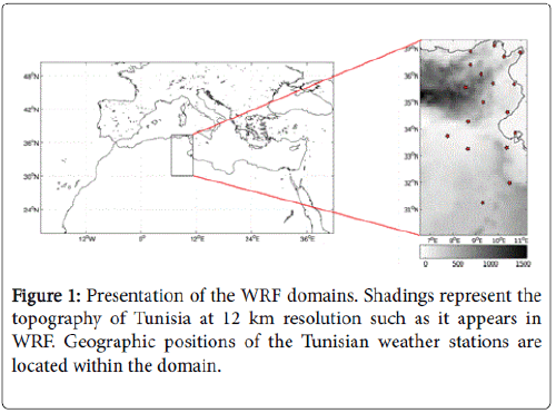
Figure 1: Presentation of the WRF domains. Shadings represent the topography of Tunisia at 12 km resolution such as it appears in WRF. Geographic positions of the Tunisian weather stations are located within the domain.
Both domains have 28 vertical levels between the surface and 50 hPa. The initial and lateral boundary conditions for the parent domain are provided by ERA-I. Lateral forcings are provided every 6 h at a 0.75° horizontal resolution and 19 pressure levels. A buffer zone composed of five grid points (1-point specified zone and 4-point relaxation zone) on the periphery of the domain is chosen and allows for a smooth transition between the model's prognostic variables and the driving reanalysis. Sea Surface Temperature (SST) fields are prescribed every 24 h by linear interpolation of monthly ERA-I SST.
The physical parameterizations chosen for the two domains include the WRF Single Moment 6-class (WSM6 [19]) cloud microphysics, the Yonsei University parameterization of the Planetary Boundary Layer (PBL, [20]), the MM5 similarity surface layer scheme [21], the Rapid Radiative Transfer Model (RRTP) scheme [22] for longwave and the Dudhia scheme for shortwave radiation [23]. The Kain-Fritschscheme [24] is used to parameterize atmospheric convection. Over the continent, WRF is coupled with Noah LSM 4-layer soil temperature, soil and canopy moistures model [25]. Surface data is derived from the 20-category Moderate Resolution Imaging Spectroradiometer (MODIS) land use data with inland water bodies [26].
The WRF run started at 0000 UTC 1 January 1991 and ended at 2400 UTC 31 December 2011, with the first year being discarded for spin-up. Temperature is archived each hour.
Analyses and comparisons are focused on daily average, minimum and maximum near-surface air temperatures (respectively Tavg, Tmin and Tmax) and are carried out at the annual and seasonal. Different verification metrics (Mean Error (ME), Root Mean Square (RMSE) and Pearson correlation coefficient (R)) are used to evaluate the WRF simulation. They are defined as:
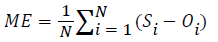 (1)
(1)
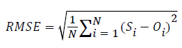 (2)
(2)
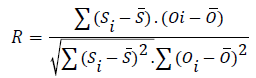 (3)
(3)
(S: simulated Temperature, O: observed temperature and N: number of grid-points)
ERA-I is however compared to the same references (E-OBS and TN_OBS) in order to know if WRF outperforms or not its driving model (i.e. whether the model improves or not the ERA-I driving temperature). Error measures are computed for common WRF, ERA-I and E-OBS landmasses (i.e after applying a mask to exclude WRF and ERA-I grid points within the Mediterranean Sea), or for the nearest grid points of gridded datasets to the Tunisian weather stations.
To better understand temperature variability and also the WRF biases, we separately examine the daily maximum and minimum near surface temperatures (Tmax and Tmin). The simulated Tmin and Tmax obtained from the WRF hourly temperature output are then compared to the same gridded datasets.
Spatial variability of temperature
Daily average temperature (Tavg): Long-term (1992-2011) climatologies of annual mean Tavg simulated by WRF and derived from ERA-I and E-OBS are computed on the basis of the annual means and are shown in Figure 2a. Overall, the spatial distribution of Tavg is heterogeneous, significantly superimposed with local orographic features and showing a clear altitudinal gradient.
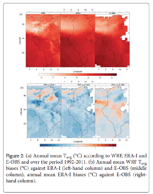
Figure 2: (a) Annual mean Tavg (°C) according to WRF, ERA-I and E-OBS and over the period 1992-2011. (b) Annual mean WRF Tavg biases (°C) against ERA-I (left-hand column) and E-OBS (middle column), annual mean ERA-I biases (°C) against E-OBS (right-hand column).
Indeed, the minimum simulated (~ 12°C) and observed (~ 14°C according to E-OBS) Tavg are observed along the main Tunisian mountain ranges, particularly along the Tunisian Dorsale (a southwestnortheast trending mountain range that mostly constitutes the eastern end of the Atlas Mountain and runs across Tunisia from the Algerian border in the west to the Cap Bon Peninsula in the east) and secondarily along the low sandstone Dahar mountain chain bisecting the south of Tunisia. Maximum simulated Tavg (~ 23°C) occurs in the west central of Tunisia particularly in the Tunisian salt depressions (the Chotts region), and south of the country on the margins of the Sahara (Grand Erg Oriental) and is in good agreement with the comparing datasets.
Figure 2b shows the spatial distribution of the 20-year average annual Tavg biases. Near-surface temperature is slightly overestimated by WRF over the north of the country. Nonetheless, the model underestimates temperature mainly along the aforementioned Tunisian mountain ranges where the cold bias can reach ~ -4°C eventually denoting strong orographic forcing, and less intensively elsewhere. Similar findings are reported by [11] for the North Western Mediterranean Basin where WRF (driven by ERA-40) particularly underestimates surface temperature along the Pyrenees. When compared to E-OBS, ERA-I slightly overestimates/underestimates air temperature in the center of Tunisia/south of the Tunisian Dorsale. Mean annual errors are summarized in Table 1.
| Model | Ref | Annual | DJF | MAM | JJA | SON | ||||||||||
|---|---|---|---|---|---|---|---|---|---|---|---|---|---|---|---|---|
| ME (°C) | RMSE (°C) | R | ME (°C) | RMSE (°C) | R | ME (°C) | RMSE (°C) | R | ME (°C) | RMSE (°C) | R | ME (°C) | RMSE (°C) | R | ||
| WRF | ERA-I | -1.02 | 1.28 | 0.95 | -1.46 | 1.62 | 0.91 | -0.97 | 1.20 | 0.97 | -0.83 | 1.37 | 0.94 | -1.08 | 1.32 | 0.93 |
| E-OBS | -1.12 | 1.28 | 0.97 | -2.15 | 2.36 | 0.84 | -0.93 | 1.08 | 0.98 | -0.29 | 0.9 | 0.96 | -1.35 | 1.53 | 0.95 | |
| TN_OBS | -1.32 | 1.68 | 0.89 | -1.8 | 1.95 | 0.81 | -1.48 | 1.1 | 0.93 | -1.28 | 1.84 | 0.9 | -1.2 | 1.65 | 0.87 | |
| E-OBS | -0.1 | 0.57 | 0.97 | -0.69 | 0.97 | 0.94 | 0.04 | 0.6 | 0.98 | 0.58 | 1.1 | 0.95 | -0.4 | 0.63 | 0.97 | |
| ERA-I | TN_OBS | -0.82 | 1.43 | 0.89 | -0.6 | 1.22 | 0.79 | -0.83 | 1.5 | 0.88 | -1.3 | 1.86 | 0.82 | -0.8 | 1.38 | 0.85 |
Table 1: Annual and seasonal Tavg errors.
Pearson's correlation coefficients quantifying the spatial matching between WRF and the comparing datasets are also listed in same table. Results show that ERA-I roughly performs better than WRF as indicated by the lower values of ME and RMSE. This result is somewhat expected since various surface observations are assimilated within the ERA-I reanalysis system. The high correlation coefficients between WRF and the other datasets (e.g., R = 0.97 with regard to EOBS) denote the good ability of the model in correctly reproducing temperature spatial variability.
Spatial distributions of seasonal mean Tavg climatologies from WRF, ERA-I and E-OBS are displayed in Figure 3. Seasons are defined as winter [December–January–February (DJF)], spring (MAM), summer (JJA), and autumn (SON). The atitudinal temperature gradient prevails throughout the year. Minimum simulated Tavg (~ 3°C) is in fact recorded in DJF over the Tunisian Dorsale, while the maximum (~ 34°C) is registered in JJA over the land depression of “Chott el- Gharsa” which constitutes the lowest altitudes of Tunisia (~ -17 m).
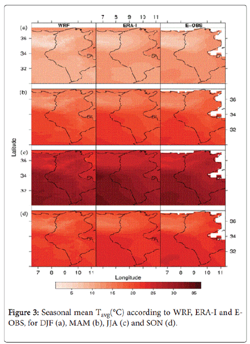
Figure 3: Seasonal mean Tavg(°C) according to WRF, ERA-I and EOBS, for DJF (a), MAM (b), JJA (c) and SON (d).
Seasonal WRF biases (Figure 4) reveal a moderate seasonal dependency. From one season to another, the spatial distribution of the biases remains roughly similar, the main differences concerning the magnitude of the errors. This magnitude itself depends on seasons, particularly for JJA when the hot biases north of Tunisia are strongest. ERA-I, compared to E-OBS, largely overestimates JJA temperature (hot bias reaching 4°C) in the center and south of Tunisia. Seasonal errors are listed in Table 1, showing that the largest WRF errors occur in DJF. The model is however closer to ERA-I then to the observational datasets in DJF (the lowest/highest spatial correlations/RMSE against observation are indeed obtained in winter).
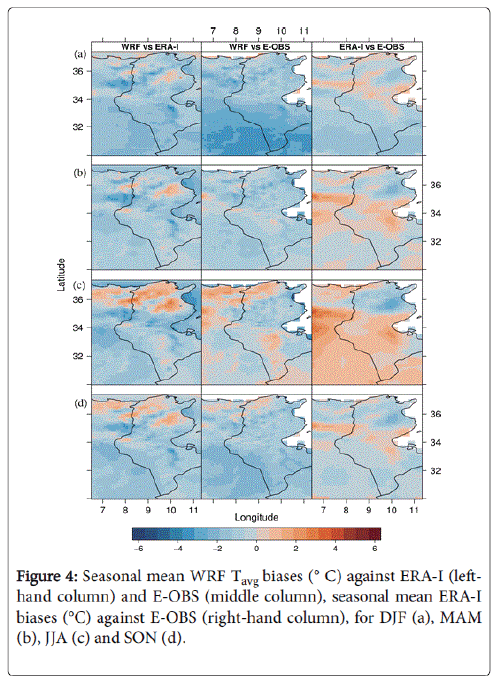
Figure 4: Seasonal mean WRF Tavg biases (° C) against ERA-I (left hand column) and E-OBS (middle column), seasonal mean ERA-I biases (°C) against E-OBS (right-hand column), for DJF (a), MAM (b), JJA (c) and SON (d).
Contrary results are obtained in JJA when WRF is, on the one hand, much closer to observation (R = 0.96 and RMSE = 0.9°C with regard to E-OBS) and slightly outperforms its driving model, on the other hand. This WRF seasonal behavior can be explained by the synoptic patterns. In DJF large scale forcing is indeed prevailing (intense prevailing westerlies), temperature is then constrained by large scale forcing (ERA-I). The connection between wintertime Tunisian climate and large-scale patterns is particularly verified for observed precipitation [27]. Contrariwise, the synoptic forcing is weak in summer, anticyclonic conditions are in fact predominant over the Mediterranean Basin [28] and the model then could be more responding to strong local (small-scale) forcings and thus better capturing details of the regional climate.
Daily maximum and minimum temperatures
Annual and seasonal spatial patterns of simulated, analyzed and observed 20-years average Tmin and Tmax (not shown) over landmasses are in agreement with the broad altitudinal pattern of the Tunisian mean temperatures.
A seasonal sea-land thermal contrast can however be noticed for both Tmin and Tmax. Indeed, Tmin (ranging in WRF from ~1°C to ~26°C) is higher over the sea (particularly over the Gulf of Gabeseast of Tunisia) then over landmasses in all seasons, excepting in JJA when the maximum occurs in the Chotts depression.
The opposite pattern is observed for Tmax (ranging in WRF from ~7°C to ~41°C) being lower over the sea in all seasons, excepting in DJF when the minimum occurs along the Tunisian Dorsale. Annual correlation coefficients between WRF and the comparing datasets (listed in Tables 2 and 3) are higher for Tmax than for Tmin. Similar findings are reported by other authors who used WRF to downscale temperature over Portugal [9] and over the US North pacific [29].
| Model | Ref | Annual | DJF | MAM | JJA | SON | ||||||||||
|---|---|---|---|---|---|---|---|---|---|---|---|---|---|---|---|---|
| ME (°C) | RMSE (°C) | R | ME (°C) | RMSE (°C) | R | ME (°C) | RMSE (°C) | R | ME (°C) | RMSE (°C) | R | ME (°C) | RMSE (°C) | R | ||
| WRF | ERA-I | -0.97 | 1.53 | 0.88 | -0.88 | 1.39 | 0.8 | -0.82 | 1.17 | 0.95 | -1.08 | 1.9 | 0.9 | -1.24 | 1.93 | 0.79 |
| E-OBS | -0.54 | 1.01 | 0.91 | -0.92 | 1.45 | 0.77 | -0.46 | 0.82 | 0.97 | -0.18 | 1.17 | 0.9 | -0.73 | 1.45 | 0.83 | |
| ERA-I | E-OBS | 0.43 | 0.83 | 0.95 | -0.04 | 0.78 | 0.89 | 0.36 | 0.74 | 0.97 | 0.9 | 1.41 | 0.95 | 0.51 | 0.89 | 0.95 |
Table 2: Annual and seasonal Tmin errors.
| Model | Ref | Annual | DJF | MAM | JJA | SON | ||||||||||
|---|---|---|---|---|---|---|---|---|---|---|---|---|---|---|---|---|
| ME (°C) | RMSE (°C) | R | ME (°C) | RMSE (°C) | R | ME (°C) | RMSE (°C) | R | ME (°C) | RMSE (°C) | R | ME (°C) | RMSE (°C) | R | ||
| WRF | ERA-I | -1.5 | 1.86 | 0.95 | -1.92 | 2.15 | 0.89 | -1.86 | 1.94 | 0.96 | -1.2 | 1.87 | 0.92 | -1.25 | 1.63 | 0.94 |
| E-OBS | -1.54 | 1.77 | 0.95 | -2.47 | 2.57 | 0.94 | -1.56 | 1.84 | 0.96 | -0.81 | 1.59 | 0.92 | -1.56 | 1.73 | 0.96 | |
| ERA-I | E-OBS | -0.04 | 0.96 | 0.95 | -0.56 | 0.79 | 0.97 | 0.3 | 1.12 | 0.96 | 0.32 | 1.54 | 0.92 | -0.31 | 0.91 | 0.96 |
Table 3: Annual and seasonal Tmax errors.
Spatial patterns of seasonal WRF and ERA-I Tmin and Tmax mean biases with regard to E-OBS are respectively shown in Figures 5 and 6. These patterns are broadly consistent with those of Tavg previously described.
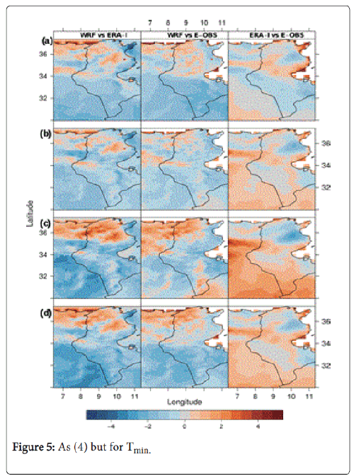
Figure 5: As (4) but for Tmin.
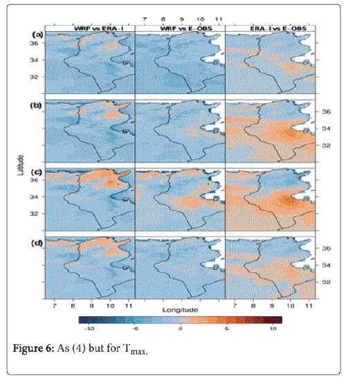
Figure 6: As (4) but for Tmax.
The largest ERA-I errors concern Tmin and are occurring in summer. WRF particularly underestimates Tmax in DJF when the cold biases are prevalent and can locally exceed -10°C. Seasonal errors (listed in Tables 2 and 3) show indeed that the largest WRF errors are obtained in DJF and mostly concern Tmax (RMSE ~ 2.6°C). WRF Tmin shows a slight improvement on ERA-I only in summer. However, ERAI always performs better than WRF (particularly in DJF and less in JJA) when reproducing the Tmax spatial variability.
Temporal variability
Figure 7a shows the interannual variability of WRF, ERA-I and EOBS Tavg spatially averaged over the landmass grid-points of the domain. A good agreement between ERA-I and E-OBS is noteworthy supporting the relevance of this reanalysis product. Concerning WRF errors, in spite of a systematic cold bias prevailing throughout the whole simulation period (reaching a maximum of -1.36°C against EOBS), the year-to-year variations of Tavg is well reproduced by the model. Interannual correlation coefficients are indeed very high against ERA-I (R = 0. 95) and E-OBS (R = 0.93).
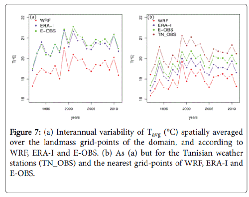
Figure 7: (a) Interannual variability of Tavg (°C) spatially averaged over the landmass grid-points of the domain, and according to WRF, ERA-I and E-OBS. (b) As (a) but for the Tunisian weather stations (TN_OBS) and the nearest grid-points of WRF, ERA-I and E-OBS.
Compared to the Tunisian stations (Figure 7b), all gridded datasets underestimate temperature. The maximum bias is recorded in WRF and ranges from -1 to -1.7°C.
Long-term mean annual cycles of Tavg in WRF and the comparing datasets are plotted in Figure 8a for the landmasses of the whole domain and in Figure 8b for TN_OBS and the nearest grid points of gridded datasets to the local weather stations.
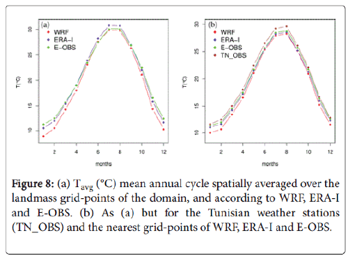
Figure 8: (a) Tavg (°C) mean annual cycle spatially averaged over the landmass grid-points of the domain, and according to WRF, ERA-I and E-OBS. (b) As (a) but for the Tunisian weather stations (TN_OBS) and the nearest grid-points of WRF, ERA-I and E-OBS.
The strong seasonality of the Tunisian temperature and its unimodal distribution are well captured by the model. The minimum and maximum simulated Tavg are respectively recorded in January (~ 9°C) and August (~ 30°C) and are in quite agreement with the other datasets. However, WRF underestimates spatially averaged Tavg throughout the whole annual cycle but mainly in winter.
In fact, WRF shows a quite strong cold bias with respect to E-OBS in DJF (especially in January when the cold bias exceeds -2°C) unlike summer when the model is notably close to E-OBS so the cold bias barely exceeds -0.2°C. Compared to TN_OBS, WRF also shows a systematic cold bias ranging from -1.8°C in February to -0.8°C in September.
Interannual variabilities of the spatially averaged Tmin and Tmax are shown in Figures 9a and 9b. WRF systematically underestimates both Tmin and Tmax throughout the whole simulation period. Nevertheless, the largest errors concern Tmax, thereby ranging from -1.9°C to -1°C with respect to E-OBS. ERA-I systematically overestimates Tmin unlike Tmax being in perfect agreement with the observation (R = 0.98).
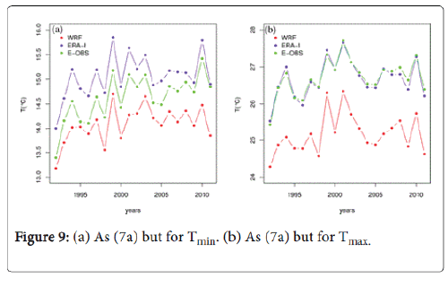
Figure 9: (a) As (7a) but for Tmin. (b) As (7a) but for Tmax.
Mean annual cycles of Tmin and Tmax are plotted in Figures 10a and 10b. Consistently with our previous findings, the main WRF errors concern Tmax and occur in wintertime, particularly in January when the systematic cold bias against E-OBS reaches its maximum (~ -3°C).
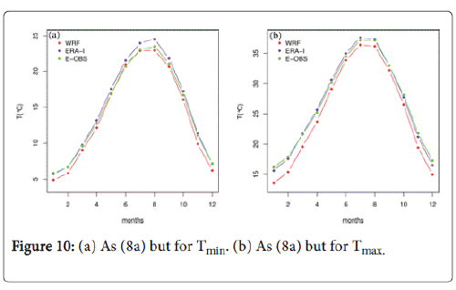
Figure 10: (a) As (8a) but for Tmin. (b) As (8a) but for Tmax.
The model Tmin is slightly underestimated against E-OBS except in June when WRF marginally overestimates temperature (bias ~ 0.2°C). Furthermore, WRF Tmin is rather in better agreement with E-OBS in JJA pointing out again the important role of regional small-scale processes being resolved by the regional model in summer. Contrariwise, the main ERA-I errors concern Tmin being overestimated in summer (a hot bias reaching ~ 1°C in August).
Our results may suggest that the WRF errors are not inherited from its driving model but are rather internal to the model itself. Indeed, underestimation of the daily average temperature seems to be a consequence of systematic underestimation of Tmax (mainly in winter) and less of Tmin, which is not verified in ERA-I. Underestimation of temperature then could be linked to deficiencies in the model parameterizations of diurnal/nocturnal physics that particularly control Tmax / Tmin [29]. The surface radiation budget (latent and heat fluxes at the surface), the PBL physics as well as the downward/ outgoing shortwave / longwave radiations at the top of the atmosphere are physical processes that strongly impact Tmax / Tmin. Evaluating the capability of WRF in simulating these processes is beyond the scope of this study.
The present study contributes for the first time to the evaluation of a near-surface air temperature simulation over Tunisia at 12 km spatial resolution. A current state-of-the-art non-hydrostatic regional (WRF) model driven by the most recent ECMWF climate reanalysis (ERAInterim) has been used to downscale temperature spatial and temporal variabilities over a 21-year long period (1991-2011). Analyses of the simulation are carried out at the annual and seasonal timescales and the WRF skills in simulating daily average (Tavg), maximum (Tmax) and minimum (Tmin) temperatures are assessed against gridded climatological datasets (ERA-I and E-OBS) and against high-quality in-situ data from 18 Tunisian weather stations. Overall, the model proves good performances in reproducing the spatial variability of mean annual and seasonal temperatures showing significant topographic signatures. Indeed, WRF correctly captures the minimum temperatures always recorded along the main Tunisian mountain ranges (particularly the Tunisian Dorsale), as well as the maximum mainly occurring in the salt chott depressions. Temporal variability of temperature is satisfactorily reproduced by WRF, despite cold biases obtained for Tavg, Tmin and Tmax, and systematically reproduced throughout the whole simulation period or the mean annual cycle. WRF tends indeed to underestimate temperature especially in DJF when the strongest cold biases are obtained and are mostly linked to an underestimation of Tmax. Results also show that the model skills depend on seasons. In fact, WRF is closer to its driving model in winter then to observation, unlike summer when WRF is notably in good agreement with E-OBS and it exclusively (but slightly) outperforms ERA-I when simulating Tavg and Tmin. This model seasonal behaviour could be linked to the Mediterranean (generally the mid-latitudes) large-scale atmospheric patterns. In winter, the synoptic forcing is active (intense westerlies) and the model then could be constrained by the ERA-I forcing. Contrariwise in summer, the low synoptic forcing could enhance the model freedom in developing its own climate thus allowing it to better capture details of the regional climate. ERA-I errors are quite different from WRF since they mainly concern Tmin being overestimated in JJA, then suggesting that the WRF errors are not inherited from its driving model but could rather be linked to deficiencies in the regional model, especially in the model parameterizations of physical processes (surface radiation budget, PBL physics and downward/outgoing shortwave / longwave radiations at the top of the atmosphere) that have a large impact on daytime / nighttime temperatures. A further study focusing on evaluating the capabilities of WRF in simulating these physical processes and also investigating other physical options seems to be worthy in order to better understand the origin of the WRF errors. Finally, this study presents a high-quality climatological dataset which can be used as reference for climate impact studies.
We wish to thank anonymous reviewers for their constructive comments that helped improve the paper. WRF was provided by the University Corporation for Atmospheric Research website (for more information see http://www.mmm.ucar.edu/wrf/users/download/). ERA-Interim data were provided by the ECMWF. Calculations were performed using HPC resources from DSI-CCUB, université de Bourgogne. We acknowledge the E-OBS dataset from the EU-FP6 project ENSEMBLES (http://ensembles-eu.metoffice.com), and the data providers in the ECA&D project (http://www.ecad.eu) and the NCDC (http://www.ncdc.noaa.gov/) for making available the Tunisian weather station data.