Research Article - (2015) Volume 3, Issue 1
Keywords: Neural networks; Climate; Surface ozone; Public health; Air quality
Surface ozone (O3) is one of the most important pollutants in troposphere. Its concentration in any given area is the result of the combination of its formation, transport, destruction and deposition. The O3 sources include: [1] photochemical reactions involving its precursors (volatile organic compounds and nitrogen oxides) with natural or anthropogenic origin; [2] downward transport from stratosphere; [3] long-range transport (intercontinental) of ozone from distant pollutant sources [1,2]. The increase of precursors’ emissions due to the economic development of many countries in the world led to the rise of the surface O3 concentrations [3-6]. Consequently, a public concern about its negative effects on human health, climate, vegetation and materials it has been observed [7-9].
About the human health protection, several studies were implemented to predict the O3 concentrations [10-12]. The statistical models are the most commonly used ones, due to the complexity of the chemical chain reactions that are associated to O3 formation and destruction. In this context, linear and nonlinear models have been applied to predict the concentration of this air pollutant. Multiple linear regression, principal component regression, quantile regression, among others, are a few examples of linear models [13-15] and on the other hand, artificial neural networks are the nonlinear models most commonly used [12,16-20]. Evolutionary procedures to determine predictive models were also applied, which include threshold autoregressive models optimized by genetic algorithms (GAs) and genetic programming models [21,22]. Moreover, in several research fields, GAs have been also applied to optimize data division, the weights or the structure of the artificial neural networks [23-26].
Information on daily levels of ozone (O3) were obtained from the Department of Physics of UFMS. The Ozone Analyzer which was used to perform the measurements has the working principle of the absorption of ultraviolet radiation by ozone molecule. The analyzer is installed near Campo Grande, away from local resources. The measurements are performed continuously 24 hours per day, and every 15 minutes, values are given of the ozone concentration. Then, when the arithmetic mean was calculated per day, it was assumed that this estimate was representative of air pollution in the city of Campo Grande. Information about rainfall, average temperature and relative humidity were obtained from Embrapa — Gado de Corte — Campo Grande.
In this study, we performed a descriptive analysis of variables which subsequently were associated with ozone concentration data, the rainfall climatic variables, maximum temperature, relative humidity and wind speed, from the period of 2004 to 2010.
Artificial neural networks
ANN can perform several functions such as classification, regression, association and mapping tasks [27-29]. They have a wide range of applications including adaptive control, optimization, medical diagnosis, decision making, as well as information, signal and speech processing [30]. ANN models are characterized by: (1) a set of processing neurons (also designated by nodes), (2) a pattern of connectivity among neurons, (3) an activation function for each neuron and (4) a learning rule. The processing neurons are distributed in layers: (1) input layer (first layer), (2) output layer (last layer) and (3) hidden layers (layers between the input and the output layers). The neurons in different layers are linked by synapses (each one storing a weight value) and the way which these linkages are done defines the structure of the network. These models were described in more detail by [29,31].
In this study, a feed forward ANN with three layers was applied to predict surface ozone concentrations with five input variables (O3, T, RH, speed, precipitation). A linear function was used as activation function of the output neuron. Concerning the hidden neurons, four functions were tested: sigmoid, hyperbolic tangent, inverse and radial basis. The early stopping method (training procedure is stopped when an increase of validation error is observed) was applied to try to avoid the over fitting.
Daily data were stored between January — 2004 and December — 2010, and the total were divided into a training group (2/3) and a test group (1/3). Ozone observed data were necessary for training and validation of the results.
The program for training and testing ANN was developed with Matlab software. Aiming the desired map, a lot of net topologies of the Feed Forward Multilayer Perceptron were tested with variations of the numbers of neurons of the intermediate layers. Since the air temperature, humidity, rainfall, wind velocity and the transport fleet are the main factors that influence the estimative of ozone concentration, its maximum, minimum and average values were used as input data in ANN. In the intermediate layer were used activation functions of tansigmoid type and in the output layer were used activation functions of linear type, featuring this neural net as a universal approximator of functions. The data standardization were made depending to the kind of activation function in the output layer of the RNA, this procedure became necessary. The software Matlab offers two forms of data standardization in an interval [-1,1] and with average=0 and variance=1 and finally the total data were divided in 2/3 consecutive for training and 1/3 for validation.
Considering that, in the beginning of training, the free parameters are randomly created and that these initial values could influence in the final result of the training, each net architecture was trained ten times, being selected that one presented the highest value of determination coefficient (R2). This coefficient was calculated from the data of the observation of the ozone concentration in the test sample and the respective values estimated by ANN.
Aiming the desired map, were trained a lot of net topologies, varying the number of neurons, activation functions in the intermediate layers, as well the numbers of the interactions (Table 1).
| Parameter | Value |
|---|---|
| Number of neurons in the intermediate layers | 1 to 5; 5 to 10 |
| Activation functions in the intermediate layers | Sigmoid Logistic; Sigmoid Hyperbolic Tangent |
| Number of cycles | 50; 100; 200; 500 |
Table 1: Parameters tested in the training of the RNAs.
The ozone values estimated by the ANN were compared with the numbers calculated by the accumulated percentage error, the Root Mean Square Error (RMSE), the exactitude coefficient of Willmot (d) and the performance index (c).
The RMSE was calculated from the equation1.
 (1)
(1)
According to Camargo and Sentelhas [32], the following statistics indicators are considered to correlate the values estimated with the measures: exactitude – index of Willmott “d”; and of trust or performance “c”. The exactitude, related to the detachment of the estimated values in relation to the observed ones, is given statistically by the agreement index proposed by Willmott [31]. Its values varies from zero, for no one agreement, to 1, for the perfect agreement. The index is given by the equation 2:
 (2)
(2)
Being: Pi = estimated value; Oi = observed value; O=average of the observed values.
The performance index “c”, presented by Camargo and Sentelhas [32], evaluates the performance of the different methods of estimative. This index gathers the indexes of precision, given by the coefficient of correlation (r) that indicates the degree of dispersion of the obtained data in relation to the average, ie, the random error and of the agreement “d”. The index “c” is calculated according the equation 3.
C = r.d (3)
Camargo and Sentelhas [32] proposed one criterion to interpret the performance of the estimative methods by the index “c”, presented in the Table 2.
| C Value | Performance |
|---|---|
| >0.85 | Great |
| 0.76a 0.85 | Very good |
| 0.66a 0.75 | Good |
| 0.61a 0.65 | Average |
| 0.51a 0.60 | Tolerable |
| 0.41a 0.50 | Bad |
| Terrible |
Table 2: Criterion of interpretation of the estimative performance of concentration of surface ozone.
After the developing of the training algorithm of the ANN and the realization of analyses of the available climate data and the training algorithms, it was obtained an ANN capable of estimate, in a satisfactory mode, the concentration of surface ozone. This estimate is realized by mapping the relation between the maximum, average and minimum temperature data, maximum, average and minimum related humidity, wind speed, rainfall, the numbers of automotive vehicles that were counted as input and the concentration of reference ozone that is the desired output.
The ANN selected presented the best performance with the minimum configuration possible. This configuration is composed of one input layer with three variables, two intermediate layers each one with 4 and 2 artificial neurons, respectively, and one neuron in the output layer. The activation function of Sigmoid Hyperbolic Tangent type was adopted for the neurons in the intermediate layer. Generally, the trained nets presented better performances with smaller numbers of cycles with the ANN selected reaching better efficiency in 200 cycles. Beyond this it was verified that the nets with more than 200 cycles presented “memorization” problems.
The annual average value was c=0.81 with a great performance and an annual monthly average of performance equal to 0.79.
Table 3 presents the values of the performance index (c) and of the root mean square error (RMSE) to the ANN’s. Lowest values of RMSE associated with highest values of “c” indicate the performance of the methodology in the estimate of ozone concentration from the collected data.
The ANN’s developed generally presented a good performance, except in the month of July, when they presented statistics index RMSE of -0.32, presenting values of “c” with a terrible performance. The concentrations of ozone presented four months of great performance, as shown in Table 3.
| Month | [O3] obs | [O3] est | RMSE | C |
|---|---|---|---|---|
| Jan | 10.32 | 13.07 | -0.27 | 0.88 |
| Feb | 12.08 | 13.55 | -0.12 | 0.88 |
| Mar | 13.28 | 14.34 | -0.08 | 0.84 |
| Apr | 13,88 | 14.08 | -0.01 | 0.83 |
| May | 14.66 | 11.40 | 0.22 | 0.73 |
| June | 14.93 | 15.54 | -0.04 | 0.69 |
| July | 15.54 | 20.50 | -0.32 | 0.56 |
| Aug | 24.29 | 24.57 | -0.01 | 0.87 |
| Sep | 29.69 | 26.30 | 0.11 | 0.86 |
| Oct | 26.79 | 21.19 | 0.21 | 0.79 |
| Nov | 21.20 | 19.84 | 0.06 | 0.82 |
| Dec | 16.10 | 14.49 | 0.10 | 0.68 |
Table 3: Statistics indicators of the adjust between the values observed of the ozone and the values estimated by then RNA, monthly average relative error, values of “c” from January of 2004 to December if 2010.
The ANN’s performance was very good, mainly due to lots of data used in its training, making its learning easier. It also contributed to the very good performance the fact that different architectures were tested in the network, i.e., different numbers of layers, algorithms of learning, number of cycles, etc.
Some works like [32,33], evaluated many architectures for the ANN’s, obtaining exceptional performances. It was emphasized that the number of cycles used in the training of the ANN’s was high, making its learning easier, reducing the possibility of memorization occurrence. The memorization leads ANN’s to present a good statistic performance (a high value of “c” and low value of RMSE), because this one is calculated based only in the sample of available data. On the other hand, the memorization would lead to serious distortions in the spatialization of the concentration of ozone extremely high or extremely low.
Analyzing the values with the ANN’s (Table 3) we can verify that the memorization didn´t occur, because were note evidenced severe deviations of the concentration of ozone estimated.
Analyzing the data of Table 2, we can verify that the average concentrations vary between 10.32 and 29.69 ppb (Table 3), with losing in the months of January, February and March, our rainfall season. The highest values were evidenced in the months of August, September and October, because it’s the time to prepare the land for planting the crops.
We observed that high values of R2 and “d” were obtained. This results were compared with those ones obtained in other studies with previsions of daily concentrations of ozone (Grivas, Chaloulakou [23] (0.60 and 0.86); Nagendra and Khare [34] (0.61 and 0.78)). The average of annual values of R² and “d” of this study were (0.8796 and 0.923798).
Figure 1 shows the graphic that compares the values observed and predicted by the model in the phase of validation. Figure 2 presents the histograms of the residues of the model evaluated in the phase of validation. A good model must have a normal distribution of the residues, i.e., the histogram of the residue must be symmetric, in the shape of a bell. To visualize the performance of the model and of the ANN, the values observed and the simulations were compared as shown in the Figure 3. The graphical shows a good adjust of the model to the observed data, both in the phase of estimation/training and in the phase of validation.
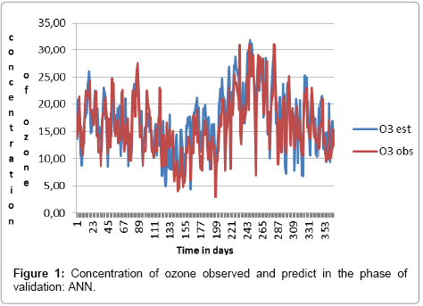
Figure 1: Concentration of ozone observed and predict in the phase of validation: ANN.
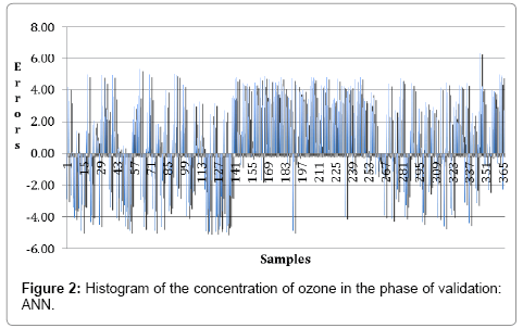
Figure 2: Histogram of the concentration of ozone in the phase of validation: ANN.
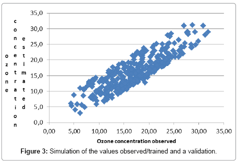
Figure 3: Simulation of the values observed/trained and a validation.
The study of the methods for the estimate ozone concentrations provides the average behavior of the parameters of study, which may be useful in prevention works of air quality, aiming the modeling work. Based on the results obtained in this work, we can conclude that:
1. The ANN’s developed for estimating the ozone concentration presented a very good statistic performance.
2. There is a need of more training of the ANN’s and variation of its architecture in order to obtain better statistic results.
3. The ANN’s developed were capable of spatialize the concentrations of ozone without the presence of greater variances in its estimate.
4. Depending on the number of variables and the complexity of the architecture result the root mean square error may decrease or increase. Correlation values can be adjusted considering the size of the data presented to the network for training, variables that may represent more adequately modeled the environment as well as the development of other network architectures, enabling forecasts for longer periods.
We would like to extend our gratitude to the many people who helped to bring this article to fruition. First of all the UFMS. Karita Cristina Francisco Veríssimo Gonçalves for the contribution in English reviewing.