Research Article - (2016) Volume 4, Issue 3
The wind-pressure relationships for tropical cyclones (TCs) in the western North Pacific are re-examined based on the aircraft data, China Meteorological Administration (CMA) TC best track data and daily NCEP reanalysis data during 1949-1987. Minimum Sea Level Pressure (MSLP) is estimated from aircraft reconnaissance, and maximum wind speeds are adjusted from the maximum wind speed at a flight level observed by Doppler radar. Using these datasets (1,766 cases), the effects of latitude, environmental pressure and intensification trend on the wind-pressure relationships was examined. Results show that adding these factors into equations that estimate the minimum pressure given a fix maximum wind speed with greater accuracy than current methodologies. The environmental pressure and latitude produce the greatest improvements, with small additional improvements form development rate and translation speed. This new wind-pressure relationship can be used easily both operationally and in postanalysis.
Keywords: Wind-pressure relationships; Tropical cyclones; Western North Pacific; Tropical Cyclone (TC)
Tropical Cyclone (TC) intensity is defined by the maximum wind speed near TC center at standard 10-m height and the Minimum Sea Level Pressure (MSLP) at TC center. The relationship between the MSLP and maximum wind speed are used both operationally and for constructing a consistent climatology of TC intensity. Over the western North Pacific, aircraft reconnaissance missions covered the TC data period from 1949 to 15 August 1987 [1]. After that, the intensity estimation of TCs in the sparse-data open oceans mainly relied on the satellite interpretation like Dvorak [2,3]. The classical Dvorak [2,3] developed a Current Intensity (CI) estimates that can be determined subjectively or objectively using satellite images. The CI number is directly related to MSLP. The wind-pressure relationship provides a critical analysis tool for obtaining the maximum wind speed based on MSLP. The actual practice of Dvorak technique varies in different operational centers. Some centers use Dvorak technique to estimate the maximum wind speed, and then use wind-pressure relationship to obtain the MSLP [4]. Therefore, the wind-pressure relationship is essentially in the assessment of TC intensity.
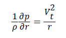
Many wind-pressure relationships were derived based on the cyclostrophic wind equation:
 (1)
(1)
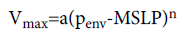
Where Vt is the tangential wind, r is the radius, p is pressure, ρ is density. A loose approximation was applied in the actual practice; the relationship was given in the form of
 (2)
(2)
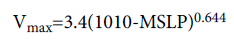
Where Vmax is the maximum wind, penv is the environmental pressure, a and n are empirical constants. The relationships were changed by varying the values of a and n [5-11]. Among these relationships, the most widely used in the west North Pacific was derived by Atkinson and Holliday [10] (here after AH1977):
 (3)
(3)
Which was used at the Joint Typhoon Warning Center (JTWC) before 2007? Aside from the development of CI number, Dvorak [2,3] suggested a table describing the wind-pressure relationship, which was used in some operational centers such as the National Hurricane Center (NHC). The wind-pressure suggested by Koba et al. [12] was used in the northwest Pacific by the Regional Specialized Meteorological Center (RSMC)-Tokyo Typhoon Center.
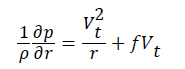
Current studies pointed that TCs are well approximated by the gradient wind balance [13,14]:
 (4)
(4)
Where f is the Coriolis parameter. Based on the wind balance, Knaff and Zehr [15] developed a comprehensive reconsideration of windpressure relationship, which considered the effect of TC size, latitude, translation speed, and environmental pressure on the relationship:
Where Vsrm is the maximum winds with translation speed removed, S is TC size, φ is latitude. Holland [16] presented a new technique for the wind-pressure relationship. Together with a method of objectively determining a derivative of the Holland b parameter, which relates directly to surface winds and varies with the pressure drop into the cyclone center, intensification rate, latitude, and translation speed. The relationships of Knaff and Zehr [15] and Holland [16] provide a realistic scatter in the maximum wind speed for a given MSLP, which are better than traditional approaches that provide a unique wind for each central pressure.
Since the recent studies related to the wind-pressure relationship by Knaff and Zehr [15] and Holland [16] are based on the best-track data and aircraft data for TCs primarily in the Atlantic, the wind-pressure relationship for TCs in the western North Pacific are need to be examined. The next section presents the data used; Section 3 discusses the effect of several factors on the wind-pressure relationship; Section 4 develops a new wind-pressure relationship; and the conclusions are presented in section 5.
Datasets
The aircraft data are used to decide the TC maximum wind speed and during 1949-1987 in the west North Pacific, which was maintained in China Meteorological Administration (CMA) Typhoon Yearbook. Each aircraft intensity fix has a time, location, MSLP, surface maximum wind, maximum winds at a flight level, and the diameter of TC eye.
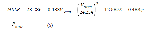
The wind speed at a flight level were observed by Doppler Radar, with the error less than 1.5 m/s, which is more reliable than the surface wind speed, which was estimated by the observer on the plane subjectively. Firstly, the surface maximum wind speed (Vmax) were extrapolated from the maximum wind speed at a fight level based on the adjustment factors suggested by Franklin et al. [17]. Samples are selected in this study when the difference between Vmax and the maximum wind observed subjectively is less than 10 m/s, and Vmax is larger than 17.2 m/s, which results in 1766 samples. The distribution of all samples is shown in Figure 1.
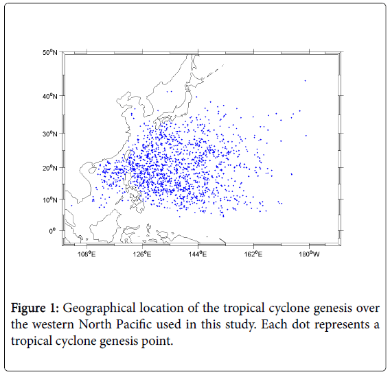
Figure 1: Geographical location of the tropical cyclone genesis over the western North Pacific used in this study. Each dot represents a tropical cyclone genesis point.
TC translation speed and intensification trend are calculated based on best-track data from CMA. Maximum wind speeds and TC center locations are interpolated to the aircraft fix time from 6-h values in the best-track data. The value 12-h prior to the aircraft fix time is also calculated in the same manner. The 12-h intensity change and translation speed are then easily calculated.
An environmental sea level pressure for each fix time is estimated by calculating the azimuthal mean pressure in an 800-1000 km annulus surrounding TC center based on daily NCEP reanalysis data.
Latitude
The average latitude of the whole sample is 19.46°N with a largest value of 43.6°N and smallest value of 4.5°N. Latitude-based composites are constructed from fixes for regions equator ward of 15°N, between 15°N and 30°N, and greater than 30°N. This resulted in 486, 890 and 389 cases, respectively. The composites results of the latitudinal stratification (Figure 2) show that higher latitude TCs have lower pressures given the same Vmax, because the Coriolis force increases as latitude increase, requiring larger pressure gradient force to balance Coriolis force, when other variables are held constant. The pressure differences between different latitudes are larger for weaker TCs. The largest difference is 12.8 hPa with Vmax between 20 and 25 m/s. The shapes of these curves suggest that the latitude of a given TC is an important factor in determining the wind-pressure relationship.
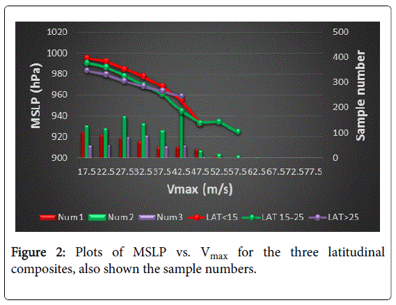
Figure 2: Plots of MSLP vs. Vmax for the three latitudinal composites, also shown the sample numbers.
Based on the gradient wind balance for TCs, we can find that the wind-pressure relationship is related to fVmax (f=2Ωsinφ), where φ is latitude. To compare the effects of these factors on the relationship, several wind-pressure models are developed. The summary error statistics for these wind-pressure models are shown in Table 1. The improvement in MLSP arising from the addition of these two predictors (φ and sinφVmax), with the larger variance explained and smaller mean absolute difference (MAD).
| Dependent variable | Independent variables | Exp-Var | Bias | MAD |
|---|---|---|---|---|
| MSLP | Vmax only | 0.625 | ~0 | 10.51 |
| Vmax+Ø | 0.638 | ~0 | 10.22 | |
| Vmax+sinØ*Vmax | 0.632 | ~0 | 10.35 | |
| Vmax+Ø+sinØ*Vmax | 0.646 | ~0 | 10.13 | |
| Vmax+Vt | 0.630 | ~0 | 10.43 | |
| Vmax+∂Vmax/∂t | 0.626 | ~0 | 10.51 | |
| Vmax+Penv | 0.658 | ~0 | 9.99 |
Table 1: Summary errors statistics for application of the wind-pressure relationship to different dependent and independent datasets in the west North Pacif. Exp-Var indicates the explained variance, MAD indicates the mean absolute difference from observations, Bais indicates the mean difference from observations.
To illustrate the effect of these two factors on the relationship clearly, a regression model is developed which represent the MSLP as a function of Vmax and latitude alone. In the model, the dependent variable is Penv-MSLP, and the Penv is 1010 hPa following the previous studies [10]. The predictors are VMAX, VMAX2, latitude and sinφVmax. The contour (Figure 3) is created using the regression coefficients applied to these four predictors.
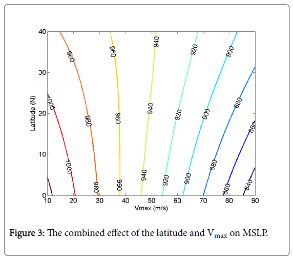
Figure 3: The combined effect of the latitude and Vmax on MSLP.
The figure shows that for a givenVmax, MSLP changes very little as the latitude of TC center increases when Vmax is between 35 m/s and 50 m/s. But for weak (Vmax<35 m/s) and strong TCs (Vmax>50 m/s), MSLP decreases significantly as the latitude increases. For given latitude, the MSLP difference between strong TCs and weak TCs is more significant when TC center locates at lower latitude.
TC translation speed
Figure 4 shows the composites results of different groups of TC translation speed. It indicates that TCs moving faster will on average have larger Vmax given the same MSLP, which is because TCs with faster speeds have been shown to have slightly larger Vmax [18] and flight-level winds [19]. In the wind-pressure models, adding the effect of TC translation speed, increases the variance explained by about 0.5%, and decreases the mean absolute error by about 0.08 hPa.
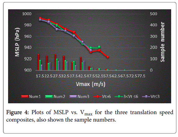
Figure 4: Plots of MSLP vs. Vmax for the three translation speed composites, also shown the sample numbers.
TC intensification trend
The composites results of different groups of TC intensification trend are shown in Figure 5 and the mean statistics with these composites are shown in Table 1. Results show that intensifying (weakening/steady) TCs have a tendency to have higher (lower) pressures. In the wind-pressure models, adding TC intensification trend did not change the variance explained and mean absolute error significantly.
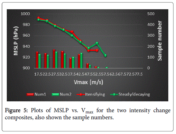
Figure 5: Plots of MSLP vs. Vmax for the two intensity change composites, also shown the sample numbers.
Environmental pressure
The mean value of Penv is 1007.4 hPa, with the standard deviation 3.13 hPa. The composite results of environmental pressure stratification (Figure 6) show that the wind-pressure relationship is clearly a function of Penv. The differences seem fairly systematic. TCs with larger Penv will have higher values of MSLP for a given Vmax. MSLP will increase as Penv increases, because the pressure gradient force should be the same when other forces are held constant. In the wind-pressure models, adding the effect of Penv, increases the variance explained by about 3.3%, and decreases the mean absolute error by about 0.52 hPa.
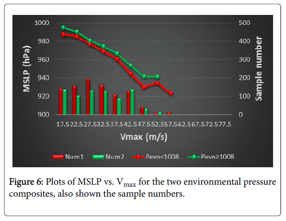
Figure 6: Plots of MSLP vs. Vmax for the two environmental pressure composites, also shown the sample numbers.
Of interest is the improvement in MSLP arising from the addition of each predictor with larger variance explained and smaller mean absolute error (Table 2).
| Independent variables | Exp-Var | Bias | MAD |
|---|---|---|---|
| Vmaxonly | 0.625 | ~0 | 10.51 |
| All factors (eqn.6) | 0.675 | ~0 | 9.68 |
| Dvorak [2] | 0.621 | 12.78 | 14.50 |
| AH [10] | 0.621 | 7.59 | 11.67 |
| Koba [12] | 0.612 | 8.32 | 12.23 |
Table 2: Summary errors statistics for application of the new windpressure relationship and Dvroak [2], AH [10] and Koba [12] in the west North Pacif. Exp-Var indicates the explained variance, MAD indicates the mean absolute difference from observations, Bais indicates the mean difference from observations.
The environmental pressure and latitude produce the greatest improvements, with small additional improvements form development rate and translation speed. An empirical wind-pressure relationship is derived considering the effect of latitude, TC translation speed, and environmental pressure. Adding the intensity trend predictor increases less than a 0.01% of the explained variance. Therefore the intensity trend is not considered in the last wind-pressure model. The resulting multiple regression equation of wind-pressure relationship is
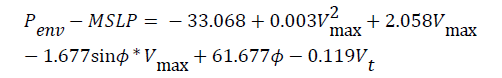 (6)
(6)
Where Ø is latitude, Vt is translation speed. The wind-pressure model explains 67.5% of the variance with a mean absolute error of 9.64 hPa and a bias of nearly zero. For comparison, the relationship table of Dvorak [2] for the western North Pacific was fit to a function Vmax=3.86(1010-MSLP)0.645, which introduces an explained variance of 62.1%, an MAE of 14.5 hPa, and a bias of 12.78 hPa. Using a similar approach, the Koba et al. [12] relationship table was fit to a function, Vmax=5.144(1010-MSLP)0.536, where Vmax is the 1-min sustained wind speed, considering the conversion value 0.93 from 10-min to 1-min averaging times. This function introduces an explained variance of 0.612, an MAE of 12.23 hPa, and a bias of 8.32 hPa. Another relationship is AH1977, Vmax=3.447(1010-MSLP)0.644 the explained variance of which is similar with Dvorak [2], while the values of bias and MAD are smaller than Dvorak [2].
These are substantial improvements in the wind-pressure model based on equation (6) than other three relationship, not only because of the larger explained variance, smaller bias, smaller MAE, but also providing a realistic scatter in the maximum wind speed for a given MSLP, which are better than traditional approaches that provide a unique wind for each central pressure.
Based on the aircraft data, CMA best-track data, and daily NCEP reanalysis data from 1949 to 1987, this study re-examined the effects of latitude, environmental pressure and intensification trend on the windpressure relationships, and then developed a new wind-pressure relationship model.
Results show that given the same Vmax, TCs which are intensifying, moving fast, located at lower latitude, and larger environmental pressure will on average have higher MSLP. The new wind-pressure model were developed by considering the effect of Vmax, latitude, translation speed and environmental pressure on the MSLP, which explains 67.5% of the variance with a mean absolute error of 9.64 hPa and a bias of nearly zero. These are substantial improvements in the new wind-pressure model than other relationship, not only because of the larger explained variance, smaller bias, smaller MAE, but also because it provides a realistic scatter in the maximum wind speed for a given MSLP.
This paper is supported by the National Natural Science Foundation of China (Grant No. 41320104007). This research was also supported by Basic Science Research Program through the National Research Foundation of Korea (NRF) funded by the Ministry of Education (2015R1D1A1A01057632).