Research Article - (2017) Volume 5, Issue 3
This paper investigated the spatio-temporal trends and homogeneity analysis of rainfall over the Komadugu-Yobe basin using data from Nigerian Meteorological Agency (NiMet), Department of National Meteorology Niger (DMN) and a 10 km resolution gridded observation data from Princeton University (PGF) for the period 1979 and 2015. The data, analysed at the annual and seasonal (wet and dry seasons) timescales, were subjected to Mann-Kendal including modified Mann-Kendall trend test after testing for autocorrelation. Test for homogeneity was performed on the data using Pettitt’s, Buishand’s, Standard Normal Homogeneity Test and van Belle and Hughes’ test. An overall homogenous trend of rainfall series was observed in the basin for all the seasons considered using van Belle and Hughes’ homogeneity trend test. The global rainfall trend increases in the dry season and decreases in the annual and wet seasons for the period of study. Pettitt’s homogeneity test for the annual and wet season rainfall series showed that change points were detected in the year 2005 for nine grids out of fifteen over the basin at 5% significant level. This study therefore, shows the importance of understanding the spatial and temporal distribution and trends in rainfall for effective planning and management of water resources in the basin.
Keywords: Rainfall; Spatio-temporal trend; Homogeneity test; Komadugu-yobe basin
There has been increased concern about water resource management in river basins due to changes in climatic conditions combined with additional anthropogenic influences [1,2]. Spatial and temporal patterns of water availability are also affected by precipitation [3]. Therefore, knowledge of precipitation patterns is of crucial importance in hydrology, e.g. to derive precipitation-runoff relationships, flood/ drought assessment and mitigation measures [4].
Different studies have investigated how changing precipitation patterns have affected the hydrological regimes of river basins. The results from these studies show that precipitation patterns in most cases dictates the hydrological regime of river basins.
Other studies [5] have observed variations in the long-term trend of precipitation patterns on both spatial and temporal scales. For example, Xu et al. [6] reported that in the 20th century, the mean annual land-surface precipitation increased by 7%-12% in the middle and high latitudes (30oN-85oN), but merely by 2% from 0o to 55oS. However, between 1910 and 1996, there was a 10% increase in annual precipitation across the United States [7]. Philandras et al. [8] found a generally negative trend in the long-term precipitation within the Mediterranean region over the period 1901-2009. In southern Italy, sub-regions of northern Africa and the western Iberian Peninsula, slightly positive trends were detected. Abbaspour et al. [9] studies in Iran noted an amplifying effect i.e. the wet regions would receive more precipitation in future, while dry regions would receive less. Bocheva et al. [10] investigated the extreme precipitation events in Bulgaria over the years 1961–2005, and reported that total precipitation was stable over the period of study. Longobardi et al. [11] utilized 211 weather stations in the Campania region of southern Italy over the period 1918- 1999. Negative trends in annual precipitation were observed in 27% and positive trends in 9% of the stations.
In Nigeria, Fasona et al. [12] stated that terrain, precipitation, and temperature are the major drivers of local climate variability in all seasons after using geographic information system and principal component analysis methods to investigate the influence of ecogeographic factors on local climate over the western Nigeria. Oguntunde et al. [13] examined the spatial and temporal patterns of monthly and annual precipitation between 1901 and 2000 and found a sharp difference in changing precipitation patterns between 1931-1960 and 1961-1990 and recorded that 1950s and 1980s are the wettest and driest decades. In northern Nigeria, Ati et al. [14] analysed precipitation data covering a period of 50 years (1953 to 2002) and reported an increase in annual trend of precipitation between 1993 and 2002. Akinsanola and Ogunjobi [15] analysed homogeneity and long-term spatiotemporal precipitation trends at the national scale in Nigeria using data from 18 stations and observed a significant increasing trend in the pre- and postmonsoon seasons. Odenuga et al. [16] investigated the hydro-climatic variability of the Hadejia-Jama’are river systems in the Komadugu- Yobe Basin (KYB) and reported a decreasing trend of rainfall from the upstream (the south of the basin) to the downstream (northern part of the basin). KYB is currently facing a conflicting balance between effectively benefiting from the available water resources and a reduction in the damages caused by the developmental projects [17]. The Hadejia River sub-basin of the KYB which is a major contributor to the Lake Chad had been subjected to tremendous exploitation of its surface water resources through the construction of several dams and large scale irrigation schemes without a prior knowledge of the trends in precipitation which regulates the water amount in the basin. This has led to the recession of Lake Chad out of Nigeria [17]. More also, there has been a decline in the occurrence of rainfall-dependent seasonal flooding which plays a vital role in maintaining and preserving the ecological system of the wetlands (Hadejia-Nguru Wetlands). This has negatively affected the practice of both flood and recession farming in the wetland region and over the entire basin [16].
The earlier cited studies suggested that spatial variability in the long-term behaviour of precipitation is dependent on regional and local characteristics. Sequel to this, relatively small-scale analyses and a check for inhomogeneity in order to avoid biases, spurious trends and erroneous interpretations from the data series used for such analyses, which is vital in practical applications of hydrology cannot be underemphasized. For this reason, this study focuses on investigating the homogeneity and trends in annual and seasonal precipitation series over the Komadugu-Yobe Basin (KYB) in the Lake Chad region between 1979 and 2015 to analyze whether or not there are significant changes in the precipitation trends as previous studies on this basin did not focus on this. This is necessary because of the enormous importance of the basin to sustaining the livelihood of the inhabitants and also its general water resources contribution to the drying Lake Chad.
Study area
The KYB is a sub-basin of the larger Lake Chad Basin. It is situated in the Sudan-Sahel zone of southeastern Niger and northeastern Nigeria covering an area of 150,000 km2 with an elevation between 294 and 1750 m above mean sea level (Figure 1). KYB covers approximately 35% of the conventional basin of Lake Chad. Ninety-five percent (95%) of the basin’s total contribution to Lake Chad is from the Nigerian sector of the KYB [16]. The Yobe River subsystem formed by the Jama’are and Hadejia tributaries creating the Hadejia-Nguru floodplain and the Komadugu Gana (or Missau) River subsystem, which historically has been seen as a tributary of the Yobe River are the two subsystems draining the basin [18]. Rainfall season is between May and October. The average annual rainfall ranges between 300 to 1200 mm [19]. The Inter-Tropical Convergence Zone (ITCZ) accounts for the highly seasonal nature of rainfall across the basin. Annual potential evaporation fluctuates between 1,800 mm and 2,400 mm across the basin, although lower rates are documented at Jos on the elevated Upland [19,20]. Two major dams (Challawa and Tiga) present in the basin supports the large scale Kano irrigation schemes while the Hadejia contributes majorly to the Kano city water supply.

Figure 1: Map of the study area.
Three drought episodes in the last century account for the basin’s climatic variability and these drought periods were characterized by considerably below average rainfall. These episodes subsequently shifted the average isohyets in the early 1950s, 1970s and particularly the 1980s southwards. As a result of this spatial overall discrepancy, there is often some temporal irregularity of rainfall in the basin [21]. The drought of the 1970s and 1980s coupled with uncoordinated water resources management and the increasing population has led to the degradation of the water resources of the basin [22].
Data
The study utilizes data from Nigeria Meteorological Agency (NiMet), Niger Direction Meteorologie National (DMN) and a 10km resolution daily gridded dataset for West Africa (PGF) developed by Princeton University between 1979 and 2015 [23]. A method for assimilating station data into the gridded dataset which has been proven to improve the quality of gridded data set was developed and tested [23-25]. This method was applied to merge fifteen station data (Table 1) from NiMET and DMN into a full gridded dataset. In this study, a subset of fifteen grid cells of daily rainfall data over the KYB has been used for the period between 1979 and 2015 (Figure 1).
| S/n | Country | Station | Lat | Long |
|---|---|---|---|---|
| 1 | Niger | Diffa | 13.314 | 12.612 |
| 2 | Niger | Goure | 13.98 | 10.3 |
| 3 | Niger | Zinder | 13.75 | 8.98 |
| 4 | Niger | Dole | 14.76 | 10.69 |
| 5 | Niger | Magaria | 12.98 | 8.93 |
| 6 | Niger | Maine-Soroa | 13.23 | 11.98 |
| 7 | Nigeria | Maiduguri | 11.81 | 13.27 |
| 8 | Nigeria | Potiskum | 11.86 | 10.77 |
| 9 | Nigeria | Katsina | 13 | 7.53 |
| 10 | Nigeria | Kaduna | 10.52 | 7.44 |
| 11 | Nigeria | Kano | 12 | 8.52 |
| 12 | Nigeria | Gombe | 13.32 | 11.17 |
| 13 | Nigeria | Nguru | 12.88 | 10.45 |
| 14 | Nigeria | Bauchi | 10.286 | 9.7 |
| 15 | Nigeria | Jos | 9.92 | 8.9 |
Table 1: List of assimilated climatic stations.
Methods
An investigation of the annual and seasonal series and trend analysis was performed on each grid cells and for the entire basin. For the seasonal analysis, the monthly rainfall data was analysed over the dry season which is between November and April and the wet season which is between May and October. Additionally, after the evaluation and subsequent setting the most probable change point, the trend analysis was done on two partial sequences before and after the change point. The following methods were used for the trend analysis;
Autocorrelation and trend test: Time-series data are often lacking serial independence. Positive serial correlation inflates the variance of the estimated time-series mean and, therefore, the time-series contains less information about the mean than a random series [26]. The serial correlation coefficient aids the validation of time-series independence. The serial independence is tested using the student’s ‘t’ test [27-29] and it is given as;
 (1)
(1)
where the test statistic t has a Student’s t-distribution with (n-2) degrees of freedom. If |t|>tα/2, the null hypothesis about serial independence is rejected at significance level α.
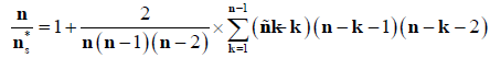
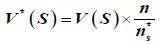
If serial correlation is found to be present in a time-series then the process of pre-whitening data may be performed. Pre-whitening a time-series removes a serial correlation component such as an autoregressive (AR) process (red noise) prior to applying the trend detection test. Modified Mann-Kendall test (MMK) pre-whitening has been used to detect a trend in a time series in the presence of autocorrelation [30]. Since pre-whitening may reduce the detection rate of significant trend in the Mann-Kendall (MK) test [31], the Modified Mann-Kendall (MMK) test [28,32] is employed for trend detection of an autocorrelated series. Only the significant values of ρk are used to calculate variance correction factor n /n*s, as the variance of S is underestimated when data are positively autocorrelated;
 (2)
(2)
where n is the actual number of observations, n* s is considered as an ‘effective’ number of observations to account for autocorrelation in data, and ρk is the autocorrelation function of ranks of the observations. The corrected variance is then computed as
 (3)
(3)
V(S) is described in Equations (5-8).
Trend test: The Mann-Kendall (MK) test [33,34] is a rank-based nonparametric test, particularly suitable for censored, missing and non-Gaussian distributed variables, which searches for a trend in a time-series without stipulating whether the trend is linear or nonlinear [35,36]. Many studies have used the Mann-Kendall test to detect trends in climatological and hydrological time-series [37-39], and this particular non-parametric test has been shown to be more powerful than some parametric tests, particularly when dealing with skewed data [40].
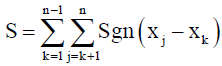
The Mann-Kendall test statistic [39,41-44], S, is defined as
 (4)
(4)
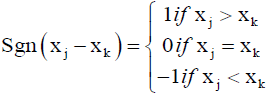
Where xj and xk are sequential data values for the time series data of length n. The test statistic represents the number of positive differences minus the number of negative differences for all the differences between adjacent points in the time-series considered and equates to the sum of the Sgn series, which is defined as
 (5)
(5)
Kendall (1975) gives the mean and variance of S, E(S) and V(S) respectively, under the null hypothesis, Ho, of randomness, given the possibility that there may be ties in the x values, as
E(S)=0 (6)
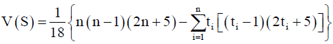 (7)
(7)
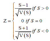
where t is the extent of any given tie. Σti denotes the summation over all ties and is only used if the data series contain tied values. The standard normal variate Z is calculated by
 (8)
(8)
Positive values of Z indicate an upward trend and negative values indicate a downward trend.
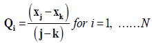
Slope test: Theil-Sen’s estimator estimates the slope of n pairs of data points [45,46] in order to assess the magnitude of the trend and this is calculated as;
 (9)
(9)
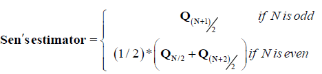
where xj and xk are values at times j and k respectively. Note, j>k. Qi is Sen’s estimator of slope which is the median of these N values. If only one data in present in each time period, then
N = n(n − 2) / 2 (10)
where n is the number of time periods. The N values of Qi are ranked by Q1≤Q2≤... ≤QN-1≤QN and
 (11)
(11)
Magnitude of percentage change: The percentage change in seasonal and annual rainfall series is computed by approximating it with a linear trend [31].
 (12)
(12)
where m is the median slope, l is the length of year and n is the mean
Homogeneity test: A climatic series is said to be homogeneous, if the observed variation is resulting from fluctuations in weather and climate exclusively. It is important to carry out different homogeneity tests. For example, standard normal homogeneity test (SNHT) is sensitive to change point towards the beginning and end of the data series while Buishand’s and Pettitt’s tests are sensitive to changes in the middle of a series.
1 Van Belle and Hughes’ homogeneity of trend test: To obtain a single global trend, this test combines data from several stations after using the Mann-Kendall statistic for each station [47,48]. Testing for the homogeneity of a global trend requires the homogeneity χ2 statistic (χ2homog) which is calculated as;
 (13)
(13)
Where ZSj is the test statistic, p is the total number of stations and ZS for the jth station obtained as;
 (14)
(14)
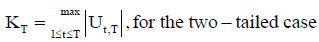
Pettitt’s test: Pettitt test is a rank-based test for detecting significant changes in the mean of time series data when the exact time of change is unknown [49]. The test is considered robust to changes in the distributional form of time series and relatively powerful compared to Wilcoxon-Mann-Whitney test, cumulative sum and cumulative deviations. Furthermore, Pettitt test has been widely adopted to detect changes in climatic and hydrological time series data [50,51].
The null and alternative hypotheses will be reformulated as follows:
Ho: The T variables follow one or more distributions that have the same location parameter.
Two-tailed test: Ha: There is a time t when there is a change of location parameter in the variables.
Left-tailed test: Ha: There is a time t when the location parameter in the variables is reduced by D.
Right-tailed test: Ha: There is a time t when the location parameter in the variable is augmented by D.
The statistic used for the Pettitt’s test is computed as follows:
Let Dij = -1 if (xi-xj) > 0, Dij = 0 if (xi-xj) = 0, Dij = 1 if (xi-xj) > 0
 (15)
(15)
The Pettitt’s statistic for the various alternative hypotheses is given by


Alexandersson’s SNHT test: To detect a change in a series of rainfall data, the standard normal homogeneity test (SNHT) [52,53] was adopted. SNHT uses series of ratios that compare the observations of a measuring station with the average of several stations. The ratios are then standardized. The standardized ratios are the series of Xi. The null and alternative hypotheses are given as;
Ho: The T variables Xi follow an N (0,1) distribution.
Ha: Between times 1 and n, the variables follow an N(μ1,1) distribution, and between n+1 and T they follow an N(μ2,1) distribution.
The Pettitt’s statistic is defined by;
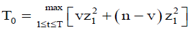 (16)
(16)
With
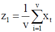
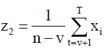
By comparing the likelihood of the two alternative models, the T0 statistic is derived. The model analogous to Ha indicates that i1 and i2 are estimated while defining the n parameter which maximizes the likelihood.
Buishand’s test: Buishand’s test is suitable for variables following any form of distribution whose properties have been mainly studied for the normal case [54]. For this study, Buishand focuses on the case of the two-tailed test and the Q statistic. For Q statistic, the null and alternative hypotheses are given by;
Ho: The T variables follow one or more distributions that have the same mean.
Two-tailed test: Ha: There exists a time t when variables change in mean.
We define
And
The Buishand’s Q statistics follows three cases;
The null and alternative hypotheses are given by;
Ho: The T variables are Homogenous.
Two-sided test: Ha: The T variables are not homogeneous.
These methods have been used previously for analysing climate data and also to investigate hydro-climatological signals of climate change and variability [11,39,55,56].
Interpolation: The spatial rainfall pattern was explored using the Inverse Distance Weighted (IDW) interpolation technique.
In IDW, weighted average of observation values is taken after which the neighborhood about the interpolated points have been identified. The weights are a decreasing function of distance of which the simplest weighting function is inverse power of the distance between points [57]:
 (17)
(17)
where d is the distance between points, p is the number of points, w is the weighting function.
The fusion of the IDW interpolated points and the Digital elevation map was carried out using the overlay function of ArcGIS.
Mean climatology
Results from the initial analysis of rainfall show that mean annual rainfall ranges from 240 mm in the northern part (Grid 1) and 1060mm in the southern part (Grid 14). This is in agreement with IUCN [19] and Thompson and Polet [21] who established that the southern part of the basin experiences more rainfall due to the southward shifts of the average isohyets. The coefficient of variation (CV) ranges from 41.49% (Grid 5) to 13.47% (Grid 11) with an average CV of 25.06% in the whole basin. This is in line with Odenuga et al. (2011), who reported such CV over the Hadeija-Jama’are basin which is a sub-basin of the KYB. However, more variations in rainfall values are established in areas with lower rainfall. This result agrees with Taxak et al. [39] who reported that zones with least variations are located on heavy rainfall zones while zones with higher variations correspond to the zone of heavy rainfall.
Figure 2a-2c represents the mean, spatially represented for the annual, wet and dry seasons respectively while Figure 2d shows the fusion of the elevation and the annual mean over the KYB. In all the seasons, rainfall increases from the north to the south due to the African monsoon which brings humidity from the Atlantic Ocean [19,21,58]. Figure 2d explains the relationship between elevation and rainfall. This explains that in KYB, the mean annual values of rainfall increases as the elevation increases, that is, from north to south [59,60].

Figure 2: Rainfall Map in Komadugu-Yobe Basin (a) Annual (b) Wet season (c) Dry season (d) Fusion of elevation and annual rainfall.
Experimental data analysis at different time scales
To identify the rainfall pattern at different time scales, the time series of annual, dry and wet season precipitation data was used. It is observed that the running mean is not resistant to local fluctuations; hence, it is pertinent to reduce the local fluctuations by fitting the time series with locally weighted scatterplot smoothing (LOWESS) regression curves [48,61,62]. Figure 3 shows the LOWESS regression curve indicating an increasing pattern of rainfall from 1979 to 2001 before the trend started decreasing for the wet and annual timescale. This could be attributed to the partial recovery of rainfall during the 1990s in the region as a result of warming of the northern Atlantic Ocean [63,64]. The increased temperature over this period as a result of the warming of the northern Atlantic Ocean draws rains during the wet season further north, therefore, increasing rainfall in the region [58]. However, for the dry season (Figure 3), there was a gradual increase in the trend of rainfall during the study period. The set back of the LOWESS regression curve is that the statistically significant trends in the time series were not accounted for [15].

Figure 3: Lowess regression line for rainfall in the basin for (a) annual, (b) dry and (c) wet seasons. Pred means prediction.
Explanatory rainfall trends at different time scales
Table 2 presents the results of the autocorrelation analysis, Z statistic and MK/MMK test for the time series between 1979 and 2015 at different time scales. On the annual scale, three grids (Grids 6, 7 and 10) were statistically autocorrelated. Grids 2, 3, 6, 7 and 14 were statistically auto correlated during the wet season and only Grid 1 was statistically autocorrelated during the dry season, all at 5% significant level. On annual time series, 5 out of 7 grid points exhibited statistically significant decreasing trend while the other two grid points (Grids 14 and 15) exhibited statistically significant increasing trend. During the wet season, 4 out of 6 grids exhibited significant decreasing trend while the other two grids (Grids 14 and 15) showed a significant increasing trend. The dry season exhibited only two grid points (Grids 1 and 4) having a significant increasing trend. All at 5% significant level.
| Grids | Seasons | ||||||||
|---|---|---|---|---|---|---|---|---|---|
| Annual | Wet | Dry | |||||||
| Z-value | Sen’s Slope | % change | Z-value | Sen’s Slope | % change | Z-value | Sen’s Slope | % change | |
| 1 | -0.23 | -2.48 | -39.63 | -0.22 | -2.53 | -40.54 | 0.38* | 0 | 0 |
| 2 | -0.25* | -8.26 | -47.71 | -0.26* | -8.39 | -49.1 | 0.15 | 0.01s | 4.37 |
| 3 | -0.23* | -4.35 | -34.5 | -0.23* | -4.35 | -34.65 | 0.17 | 0.01s | 10.61 |
| 4 | 0.02 | 0.11 | 1.11 | 0.01 | 0.07s | 0.73 | 0.25* | 0.002 | 6.46 |
| 5 | -0.23* | -4.88 | -44.22 | -0.21 | -4.89 | -44.76 | -0.2 | -0.01s | -6.73 |
| 6 | -0.26* | -8.77 | -41.43 | -0.26* | -9.47 | -45.49 | 0.13 | 0.04s | 10.04 |
| 7 | -0.18 | -4.25 | -27.58 | -0.19 | -4.45 | -29.15 | 0.16 | 0.03s | 18.91 |
| 8 | -0.25* | -2.71 | -24.5 | -0.25* | -2.64 | -24.09 | 0.04 | 0 | 0 |
| 9 | -0.15 | -2.96 | -21.11 | -0.13 | -3 | -21.68 | -0.02 | 0 | 0 |
| 10 | 0.13 | 3.14 | 13.53 | 0.1 | 2.38 | 10.55 | 0.17 | 0.36 | 58.08 |
| 11 | -0.03 | -0.33 | -1.69 | -0.04 | -0.49 | -2.55 | 0.13 | 0.09 | 26.46 |
| 12 | -0.15 | -1.52 | -9.01 | -0.14 | -1.49 | -8.98 | 0.15 | 0.06 | 23.58 |
| 13 | 0.01 | 0.01s | 0.06 | -0.02 | -0.34 | -2.34 | 0.21 | 0.07 | 35.18 |
| 14 | 0.40* | 10.34 | 40.85 | 0.37* | 9.89 | 40.82 | 0.17 | 0.58 | 53.36 |
| 15 | 0.37* | 7.14 | 29.67 | 0.38* | 6.87 | 29.43 | 0.06 | 0.19 | 25.98 |
Table 2: Mann-Kendall (Modified MK) test (at 5% level) and percentage change with autocorrelation. Bold values represent autocorrelation in rainfall series, * means significant trend, positive/negative Z means increasing/decreasing trend, s means statistically significant magnitude of change. For more information about the location of the grid cells, please see Figure 1.
Table 2 further explains the percentage changes in mean values for the annual, wet and dry seasons. It was observed that all the grids recorded changes in precipitation for all the seasons. Sen’s slope estimator determines the magnitude of statistically significant trends. Statistically significant magnitude of change was observed in the annual series (Grid 13), Wet season (Grid 4) and Dry season (Grids 2,3,5,6 and 7).
Figure 4a-4c shows that for the three time scales considered, grids 14 and 1 were consistent in having the highest rising and lowest falling trends respectively at 5% significant level. It is worthy to note that PGF which is a high resolution gridded dataset clearly reveals that the percentage of change of rainfall increases to the south of the basin. This phenomenon has not been recorded by larger scale regional studies [65,66]. This ascertained the usefulness of the PGF for regional studies. However, Figure 4d shows a positive percentage magnitude of change of rainfall at higher elevation and a negative percentage magnitude of change of rainfall at lower elevation.

Figure 4: Spatial distribution of the percentage of change (a) Annual (b) Wet season (c) Dry season (d) Fusion of elevation and annual rainfall.
Change point analysis across grids and magnitude of trend slope in rainfall series
The change point probability and detection of homogeneity of the data series using Pettitt’s test, SNHT test and Buishand’s test are discussed in this section. Pettitt’s homogeneity test for the annual rainfall series (Table 3) shows that most grids were heterogeneous and particularly, change points were detected in the year 2005 for nine grids, signifying a significant change in the mean before and after the identified change point. Most of the grids are homogenous in the dry season (Table 4) while the wet season follows the same trend as the annual series (Table 5). To find change point towards the beginning and end of the series, SNHT is applied while Buishand’s and Pettitt’s tests are sensitive to find the changes in the middle of a series. Change year in annual rainfall series is shown in Figure 5; (a) Grid 1 (b) Grid 2 (c) Grid 5 (d) Grid 9 (e) Grid 14 (f) Grid 15. Five of these six grids show a change point in 2005 while grid 15 is the only grid showing a change point in 1995. The change points recorded may be attributed to changes in instruments, observing practices, station location, station environment, satellite sensors, and network configuration and density [67-69]. It is worthy to note that grids located at the southern part of the basin (grids 14 and 15) recorded an increased annual rainfall after the change points while the grids located in the north of the basin recorded a decreased annual rainfall after the change point (Figure 5).
| Grids | Pettitt’s Test | Standard Normal Homogeneity Test (SNHT) | Buishand Test | |||||||||
|---|---|---|---|---|---|---|---|---|---|---|---|---|
| K | t | P-value | Trend | To | t | P-value | Trend | Q | t | P-value | Trend | |
| 1 | 212 | 2005 | 0.0045 | Ha | 9.25 | 2005 | 0.0271 | Ha | 8.33 | 2005 | 0.0225 | Ha |
| 2 | 258 | 2005 | 0.0001 | Ha | 20.08 | 2005 | <0.0001 | Ha | 12.27 | 2005 | <0.0001 | Ha |
| 3 | 240 | 2005 | 0.0005 | Ha | 14.95 | 2005 | 0.0004 | Ha | 10.59 | 2005 | 0.0014 | Ha |
| 4 | 130 | 1993 | 0.1885 | Ho | 4.69 | 1987 | 0.3521 | Ho | 5.88 | 1990 | 0.2036 | Ho |
| 5 | 252 | 2005 | 0.0003 | Ha | 13.75 | 2005 | 0.0058 | Ha | 10.15 | 2005 | 0.0014 | Ha |
| 6 | 270 | 2005 | <0.0001 | Ha | 19.6 | 2005 | <0.0001 | Ha | 12.12 | 2005 | <0.0001 | Ha |
| 7 | 224 | 2005 | 0.0016 | Ha | 13.53 | 2005 | 0.0008 | Ha | 10.07 | 2005 | 0.0026 | Ha |
| 8 | 174 | 2005 | 0.0323 | Ha | 5.89 | 2005 | 0.1457 | Ho | 6.64 | 2005 | 0.119 | Ho |
| 9 | 230 | 2005 | 0.0011 | Ha | 9.98 | 2005 | 0.0251 | Ha | 8.65 | 2005 | 0.0138 | Ha |
| 10 | 180 | 1990 | 0.0259 | Ha | 6.72 | 1990 | 0.1448 | Ho | 7.48 | 1990 | 0.053 | Ho |
| 11 | 68 | 2000 | 0.8709 | Ho | 4.12 | 1980 | 0.4192 | Ho | 3.08 | 1987 | 0.8908 | Ho |
| 12 | 110 | 2003 | 0.355 | Ho | 4.59 | 1979 | 0.3379 | Ho | 4.22 | 2003 | 0.5861 | Ho |
| 13 | 78 | 1998 | 0.7475 | Ho | 3.91 | 1979 | 0.4459 | Ho | 3.52 | 1998 | 0.7862 | Ho |
| 14 | 258 | 2005 | <0.0001 | Ha | 23.9 | 2005 | <0.0001 | Ha | 13.39 | 2005 | <0.0001 | Ha |
| 15 | 254 | 1995 | <0.0001 | Ha | 13.68 | 1995 | 0.0005 | Ha | 11.37 | 1995 | <0.0001 | Ha |
Table 3: Most probably change year (t) by Pettitt’s, SNHT and Buishand’s tests for the Annual season. Ho denotes Homogeneous series, Ha denotes Heterogeneous series, t denotes year of change. For more information about the location of the grid cells, please see Figure 1.
| Grids | Pettitt’s Test | SNHT | Buishand’s Test | |||||||||
|---|---|---|---|---|---|---|---|---|---|---|---|---|
| K | t | P-value | Trend | T0 | t | P-value | Trend | Q | t | P-value | Trend | |
| 1 | 212 | 2005 | 0.0001 | Ha | 16.05 | 2005 | 0.0154 | Ha | 10.97 | 2005 | 0.0004 | Ha |
| 2 | 113 | 1987 | 0.3343 | Ho | 2.01 | 1994 | 0.7202 | Ho | 4.34 | 1994 | 0.591 | Ho |
| 3 | 118 | 1990 | 0.267 | Ho | 1.71 | 1990 | 0.8826 | Ho | 3.78 | 1990 | 0.7294 | Ho |
| 4 | 136 | 2000 | 0.1128 | Ho | 7.01 | 2005 | 0.1475 | Ho | 7.25 | 2005 | 0.0718 | Ho |
| 5 | 119 | 1995 | 0.2489 | Ho | 3.3 | 1992 | 0.4424 | Ho | 5.43 | 1992 | 0.2251 | Ho |
| 6 | 105 | 1987 | 0.4202 | Ho | 1.67 | 1987 | 0.8726 | Ho | 3.57 | 2003 | 0.7787 | Ho |
| 7 | 110 | 1987 | 0.3527 | Ho | 2.14 | 1987 | 0.7394 | Ho | 3.88 | 1993 | 0.6961 | Ho |
| 8 | 98 | 1987 | 0.4635 | Ho | 2.06 | 2007 | 0.8171 | Ho | 4.01 | 2003 | 0.6672 | Ho |
| 9 | 75 | 1987 | 0.7902 | Ho | 2.94 | 1995 | 0.5409 | Ho | 5.27 | 1995 | 0.2869 | Ho |
| 10 | 120 | 2002 | 0.2596 | Ho | 4.11 | 2002 | 0.3798 | Ho | 5.97 | 2002 | 0.1966 | Ho |
| 11 | 122 | 2000 | 0.2535 | Ho | 1.36 | 2000 | 0.9185 | Ho | 3.53 | 2000 | 0.8324 | Ho |
| 12 | 122 | 2000 | 0.2531 | Ho | 0.97 | 2003 | 0.9851 | Ho | 2.84 | 2003 | 0.9414 | Ho |
| 13 | 119 | 2000 | 0.2732 | Ho | 1.81 | 2000 | 0.8487 | Ho | 4.07 | 2000 | 0.6456 | Ho |
| 14 | 138 | 2006 | 0.1413 | Ho | 3.91 | 2002 | 0.3772 | Ho | 5.82 | 2002 | 0.2251 | Ho |
| 15 | 66 | 1980 | 0.8868 | Ho | 1.45 | 1980 | 0.904 | Ho | 3.55 | 2000 | 0.8251 | Ho |
Table 4: Most probably change year(t) by Pettitt’s, SNHT and Buishand’s tests for the Dry season. Ho denotes Homogeneous series, Ha denotes Heterogeneous series, t denotes year of change. For more information about the location of the grid cells, please see Figure 1.
| Grids | Pettitt’s Test | SNHT | Buishand’s Test | |||||||||
|---|---|---|---|---|---|---|---|---|---|---|---|---|
| K | t | P-value | Trend | T0 | t | P-value | Trend | Q | t | P-value | Trend | |
| 1 | 212 | 2005 | 0.0028 | Ha | 9.34 | 2005 | 0.0261 | Ha | 8.37 | 2005 | 0.0214 | Ha |
| 2 | 262 | 2005 | 0.0001 | Ha | 20.35 | 2005 | <0.0001 | Ha | 12.35 | 2005 | <0.0001 | Ha |
| 3 | 240 | 2005 | 0.0005 | Ha | 14.08 | 2005 | 0.0007 | Ha | 10.64 | 2005 | 0.0013 | Ha |
| 4 | 124 | 1993 | 0.2298 | Ho | 4.61 | 1987 | 0.3686 | Ho | 5.79 | 1990 | 0.2172 | Ho |
| 5 | 252 | 2005 | 0.0002 | Ha | 13.64 | 2005 | 0.0059 | Ha | 10.11 | 2005 | 0.0015 | Ha |
| 6 | 268 | 2005 | 0.0001 | Ha | 20.19 | 2005 | <0.0001 | Ha | 12.31 | 2005 | 0.0002 | Ha |
| 7 | 224 | 2005 | 0.0013 | Ha | 13.98 | 2005 | 0.0006 | Ha | 10.24 | 2005 | 0.0021 | Ha |
| 8 | 174 | 2005 | 0.0313 | Ha | 5.64 | 2005 | 0.1662 | Ho | 6.51 | 2005 | 0.1299 | Ho |
| 9 | 228 | 2005 | 0.001 | Ha | 9.76 | 2005 | 0.0282 | Ha | 8.56 | 2005 | 0.0158 | Ha |
| 10 | 174 | 1990 | 0.0333 | Ha | 6.25 | 1990 | 0.2133 | Ho | 7.22 | 1990 | 0.0719 | Ho |
| 11 | 82 | 2000 | 0.7 | Ho | 5.23 | 1980 | 0.2462 | Ho | 3.4 | 2000 | 0.8105 | Ho |
| 12 | 104 | 1982 | 0.4233 | Ho | 5 | 1981 | 0.2728 | Ho | 4.24 | 1982 | 0.5837 | Ho |
| 13 | 76 | 1991 | 0.7738 | Ho | 4.34 | 1981 | 0.3511 | Ho | 3.55 | 1982 | 0.7762 | Ho |
| 14 | 260 | 2005 | 0.0003 | Ha | 23.47 | 2005 | <0.0001 | Ha | 13.27 | 2005 | <0.0001 | Ha |
| 15 | 260 | 1995 | <0.0001 | Ha | 14.16 | 1995 | 0.0001 | Ha | 11.56 | 1995 | <0.0001 | Ha |
Table 5: Most probably change year (t) by Pettitt’s, SNHT and Buishand’s tests for the Wet season. Ho denotes Homogeneous series, Ha denotes Heterogeneous series, t denotes year of change. For more information about the location of the grid cells, please see Figure 1.

Figure 5: Change year in annual rainfall series (a) Grid 1 (b) Grid 2 (c) Grid 5 (c) Grid 9 (d) Grid 14 (f) Grid 15.
In general, human activities [70,71], buildup of atmospheric dust and frequent sand storm [72], regional and global scale pattern of sea surface temperature (SST)[73], reduction in forest cover [74,75], anthropogenic activities [76] global climate shift [77], or weakening global monsoon circulation [78] may be the probable causes of the changes in rainfall.
Analysis of homogeneity of trends for the entire basin
To obtain a single global trend for the entire basin, van Belle and Hughes’ homogeneity trend test was applied to the rainfall time series data from the several grids considered during the annual, wet and dry seasons. The results in Table 6 shows that at 95% confidence level, there exist an overall homogenous trend of rainfall series in the KYB for all the seasons considered. The values of x2homogenous are 0.11, 0.28 and 0.06 for annual, dry and wet seasons respectively. There was also a statistically non-significant decreasing trend of rainfall in Annual and wet seasons while the increasing trend in dry season is statistically non-significant. In the entire basin, the wet season and annual rainfall decreased by 0.11% and 0.03% respectively while there was an increase of 46.22% in the dry season for the period of study.
| Seasons | x2homogenous | Trend | Mean | MK(MMK) | Sen's slope | % change |
|---|---|---|---|---|---|---|
| Annual | 0.11 | Ho | 601 | -0.003 | -0.005 | -0.03 |
| Dry | 0.28 | Ho | 13 | 0.17 | 0.166 | 46.22 |
| Wet | 0.06 | Ho | 588 | -0.003 | -0.018 | -0.11 |
Table 6: Homogeneity trends, MK (MMK) test, Thiel and Sen’s slope and % change over the Komadugu-Yobe Basin.
The study investigated trends and homogeneity of trends in rainfall time series for annual, wet and dry season over Komadugu-Yobe basin between 1979 and 2015. The analysis shows that the annual rainfall increases from the northern to the southern part of the basin. The Mann-Kendall statistic shows that there is a decreasing trend of rainfall in most grids over the basin for both annual and wet season while dry season exhibited an increasing trend indicating a shift in seasonal rainfall [17]. This trend was also established in the entire basin for the period of study. As a result of this, rainfall-dependent seasonal flooding phenomenon in the basin could be subdued and this will greatly reduce fishing and agricultural activities in the basin’s wetlands [18,79]. Odunuga et al. [16] already investigated the declining agricultural activities in the Hadejia sub-basin of the KYB and this was attributed principally to the decreasing rainfall, although, they pointed out other human activities like the dam construction at the upstream of the subbasin. This could lead to communal clashes among the inhabitants [80]. However, care must be taken no to run to incorrect conclusions as the observed patterns may be a swing in the 200-year cycle of the region [65,81].
The rising and falling trends of rainfall are observed at higher elevation and at lower elevation respectively. There exists an overall homogenous trend of rainfall series in the KYB for all the seasons considered. Furthermore, the result shows that rainfall series vary at both temporal and spatial scales. The variations at both scales will have a major impact on water resources management, agricultural practices and the socio-economic activity of the basin. Additionally, in attaining greater efficiency in the consumption of valuable fresh water resources in the face of drought and climate change, there is a need for adequate preparation in terms of storage, distribution and environmental services which are necessary for optimizing the fresh water resource. Operations of the upstream dams should be targeted at mimicking the natural flood regime so as to cushion the effect of droughts arising from varying precipitation regimes in the basin.
Further studies are required to verify and quantify the rainfall variations presented in statistical tests by ascertaining the physical mechanisms behind the changes.
The authors wish to acknowledge NiMET, DMN and Princeton University for providing the data used for this study. Also, we acknowledge the German Federal Ministry of Education for providing funds for this project. We also acknowledge the fruitful discussions with Dr Seyni Salack of the WASCAL competent centre, Burkina Faso. The anonymous reviewers are also acknowledged.
The Authors have read and understood the policy on declaration of interests and declare that we have no competing interests. This article does not contain any studies with human or animal subjects.