Research Article - (2015) Volume 3, Issue 1
Keywords: Wind energy potential; Wind turbine; Weibull distribution function; Wind power density; One seventh power law; Kerman province
The worldwide concern and environmental awareness of air quality created a move towards pollution free energy production such as solar and wind energies. Wind is an abundant resource available in nature that can be utilized by mechanically converting wind power to electricity. Wind turbines are especially meant for this purpose.
The gradual increase in the earth population and the increasing demand for energy from natural resources have been the major causes for man to search for an appropriate substitution for the sources of energy. Having been aware of the decrease of the earth’s energy resources, scientists have cautioned against the surplus use of energy. Moreover, environmental pollutions resulting from the burning of fossil fuels in the power stations have led to energy loss. This phenomenon is a threat to every living creature on the earth. Thus, the appropriate use of energy and the involvement of new sources of energy have been the focus of study for a long time. An appropriate solution to lower the impact of energy loss is the substitution of renewable forms of energies such as wind.
World winds hold almost around 2700 TW potential energy -25% of this energy occupies an environment of 100 meters above the ground level. It is noteworthy that 10% of this energy, i.e. 4 TW exceeds the capacity of the world’s total water energy [1].
Although Iran has been a pioneer in the use wind energy, we have yet to witness the applications of wind energy which have been extremely limited. But the remnants of the numerous windmills all over the country support our claim that undoubtedly wind energy must have been of importance.
This project attempts to discover not only potential power of wind energy but also the feasibility of using wind power at Kerman synoptic stations in Iran.
Moreover, in the process of this study, a new formula, has been obtained that can be applied for computing wind existence hours at an area.
Since wind is a vector quantity having direction and speed, it is subject to topographical and atmospheric changes. It is impossible to make an estimation of wind direction and wind speed at intervals in which wind speed is not reported. Moreover, this estimation is not error free. To reduce the impact of this error, the researcher took raw data from Tehran Meteorology Organization for a period of at least 20 years. The data reported wind direction and wind speed at Kerman synoptic stations for the consecutive years. Then wind data were converted from Knot to m/s (1 Knot=0.514 m/s).
All the graphs, tables and data in the project were analyzed by applying Excel and SPSS 17. In order to process the data the mathematical model Weibull Probability Distribution Function is used. Probability Distribution Function is the most applicable strategy to the study and calculation of wind statistics at a specific location. After the calculation of the components of this function, some parameters relating to the calculation of wind energy can be estimated.
There are several mathematical functions called probability density functions that can be applied to model the wind speed frequency curve. In wind power studies, Weibull and Rayleigh probability density functions are commonly used and widely adopted [2]. Herein Weibull distribution is used since the Rayleigh distribution is only a subset of it.
Weibull distribution function of wind speed
Wind power is proportionate to the cubic power of the wind speed and rotor’s diameter square root power [3]. Thus, wind speed is one of the most significant factors in the optimum use of wind energy.
In the calculation of wind energy, wind speed is considered a random variable which can take every quantity in a specific distance. However, practically wind speed data recorded every 3 hours at synoptic stations. The function of which is a disconnect function. In other words, the frequency distribution should be first replaced by the connected distribution function. For this purpose Weibull probability distribution function is reliable and is the most frequently used model to describe the distribution of the wind speed [4].
Weibull distribution function is a derivative of Gamma distribution and has a higher flexibility in comparison with Rayleigh distribution. It can be defined as follows:
 (1)
(1)
where V [m/s] is the wind speed, K [–] is the Weibull shape parameter describing the dispersion data and C [m/s] is the Weibull scale parameter.
Values of the two parameters, K and C, can be calculated by using the least square fitting of the data [5] i.e.
 (2)
(2)
Where
 (3)
(3)
And
 (4)
(4)
where  is the mean of wind speed classes,
  is the accumulative probability of the frequency of every mean speed classes. By quantities of X and Y, the values of A and B can be calculated using the following equation:
 (5)
(5)
 (6)
(6)
Here, A is the gradient of the equation of a straight line Y=AX+B, B is the width of the intersection of the line by the Y axis. In this equation, the relationship between A and B and the Weibull parameters K and C is as follows [6]:
 and
and  (7)
(7)
A brief presentation of the observations and measurements of wind speed at Kerman synoptic stations are shown in Tables 1-9
| I | Wind speed classes v[m/s] |
Mean of wind speed classes vi[m/s] |
Frequency fi |
Probability (iv)p |
Accumulative probability (iv)P |
Probability in Weibull model Pw (vi) |
|---|---|---|---|---|---|---|
| 1 | 0.5-1.5 | 1 | 116 | 0.004278548 | 0.004278548 | 0.0597024 |
| 2 | 1.5-2.5 | 2 | 4599 | 0.169629684 | 0.173908233 | 0.1051664 |
| 3 | 2.5-3.5 | 3 | 6671 | 0.246053408 | 0.419961641 | 0.1333364 |
| 4 | 3.5-4.5 | 4 | 4830 | 0.178149897 | 0.598111537 | 0.1430981 |
| 5 | 4.5-5.5 | 5 | 3632 | 0.133962821 | 0.732074358 | 0.1368364 |
| 6 | 5.5-6.5 | 6 | 2471 | 0.091140454 | 0.823214813 | 0.1193128 |
| 7 | 6.5-7.5 | 7 | 1675 | 0.061780761 | 0.884995574 | 0.0960548 |
| 8 | 7.5-8.5 | 8 | 1209 | 0.0445928 | 0.929588374 | 0.0719434 |
| 9 | 8.5-9.5 | 9 | 326 | 0.012024196 | 0.94161257 | 0.0503812 |
| 10 | 9.5-10.5 | 10 | 724 | 0.026704042 | 0.968316613 | 0.0331025 |
| 11 | 10.5-11.5 | 11 | 103 | 0.003799056 | 0.972115668 | 0.0204583 |
| 12 | 11.5-12.5 | 12 | 343 | 0.012651225 | 0.984766893 | 0.0119159 |
| 13 | 12.5-13.5 | 13 | 96 | 0.003540868 | 0.98830776 | 0.0065506 |
| 14 | 13.5-14.5 | 14 | 125 | 0.004610505 | 0.992918265 | 0.003403 |
| 15 | 14.5-15.5 | 15 | 97 | 0.003577752 | 0.996496017 | 0.0016721 |
| 16 | 15.5-16.5 | 16 | 32 | 0.001180289 | 0.997676306 | 0.0007778 |
| 17 | 16.5-17.5 | 17 | 19 | 0.000700797 | 0.998377102 | 0.0003428 |
| 18 | 17.5-18.5 | 18 | 19 | 0.000700797 | 0.999077899 | 0.0001432 |
| 19 | 18.5-19.5 | 19 | 1 | 0.000037 | 0.999114783 | 0.0000567 |
| 20 | 19.5-20.5 | 20 | 18 | 0.000664 | 0.999778696 | 0.0000213 |
| 21 | 21.5-22.5 | 22 | 1 | 0.000037 | 0.99981558 | 0.0000026 |
| 22 | 22.5-23.5 | 23 | 2 | 0.000074 | 0.999889348 | 0.0000008 |
| 23 | 24.5-25.5 | 25 | 3 | 0.000111 | 0.999999 | 0.0000001 |
| 1 |
Table 1: Arrangement of the measured three hourly time-series data in frequency distribution format for 1986-2011 and the probability density distributions calculated from the Weibull function at Anar synoptic station.
| i | Wind speed classes v[m/s] |
Mean of wind speed classes vi[m/s] |
Frequency fi |
Probability (iv)p |
accumulative probability (iv)P |
Probability in Weibull model Pw (vi) |
|---|---|---|---|---|---|---|
| 1 | 0.5-1.5 | 1 | 9 | 0.000326 | 0.000326 | 0.0228712 |
| 2 | 1.5-2.5 | 2 | 2665 | 0.096642 | 0.096968 | 0.0558927 |
| 3 | 2.5-3.5 | 3 | 5415 | 0.196366 | 0.293335 | 0.0891254 |
| 4 | 3.5-4.5 | 4 | 6664 | 0.241659 | 0.534994 | 0.1158754 |
| 5 | 4.5-5.5 | 5 | 4213 | 0.152778 | 0.687772 | 0.1313352 |
| 6 | 5.5-6.5 | 6 | 3085 | 0.111873 | 0.799645 | 0.1334372 |
| 7 | 6.5-7.5 | 7 | 959 | 0.034777 | 0.834421 | 0.1231778 |
| 8 | 7.5-8.5 | 8 | 2133 | 0.077350 | 0.911771 | 0.1040348 |
| 9 | 8.5-9.5 | 9 | 266 | 0.009646 | 0.921417 | 0.080687 |
| 10 | 9.5-10.5 | 10 | 1301 | 0.047179 | 0.968596 | 0.0575692 |
| 11 | 10.5-11.5 | 11 | 23 | 0.000834 | 0.96943 | 0.0378135 |
| 12 | 11.5-12.5 | 12 | 409 | 0.014832 | 0.984262 | 0.0228657 |
| 13 | 12.5-13.5 | 13 | 33 | 0.001197 | 0.985458 | 0.0127242 |
| 14 | 13.5-14.5 | 14 | 133 | 0.004823 | 0.990281 | 0.0065115 |
| 15 | 14.5-15.5 | 15 | 141 | 0.005113 | 0.995395 | 0.0030617 |
| 16 | 15.5-16.5 | 16 | 35 | 0.001269 | 0.996664 | 0.0013214 |
| 17 | 16.5-17.5 | 17 | 12 | 0.000435 | 0.997099 | 0.000523 |
| 18 | 17.5-18.5 | 18 | 38 | 0.001378 | 0.998477 | 0.0001895 |
| 19 | 18.5-19.5 | 19 | 1 | 0.000036 | 0.998513 | 0.0000628 |
| 20 | 19.5-20.5 | 20 | 32 | 0.001160 | 0.999674 | 0.000019 |
| 21 | 21.5-22.5 | 22 | 1 | 0.000036 | 0.99971 | 0.0000013 |
| 22 | 23.5-24.5 | 24 | 1 | 0.000036 | 0.999746 | 0.0000001 |
| 23 | 24.5-25.5 | 25 | 5 | 0.000181 | 0.999927 | 0 |
| 24 | 27.5-28.5 | 28 | 2 | 0.000073 | 0.99999 | 0 |
| 27576 | 1 |
Table 2: Arrangement of the measured three hourly time-series data in frequency distribution format for 1986-2011 and the probability density distributions calculated from the Weibull function at Baft synoptic station.
| i | Wind speed classes v[m/s] |
Mean of wind speed classes vi[m/s] |
Frequency fi |
Probability (iv)p |
accumulative probability (iv)P |
Probability in Weibull model Pw (vi) |
|---|---|---|---|---|---|---|
| 1 | 0.5-1.5 | 1 | 2869 | 0.036216059 | 0.036216059 | 0.1453942 |
| 2 | 1.5-2.5 | 2 | 17502 | 0.220931847 | 0.257147906 | 0.1647792 |
| 3 | 2.5-3.5 | 3 | 12974 | 0.163773842 | 0.420921749 | 0.1551221 |
| 4 | 3.5-4.5 | 4 | 17059 | 0.215339754 | 0.636261503 | 0.1326244 |
| 5 | 4.5-5.5 | 5 | 9521 | 0.120185814 | 0.756447317 | 0.1061931 |
| 6 | 5.5-6.5 | 6 | 8499 | 0.107284869 | 0.863732185 | 0.0808406 |
| 7 | 6.5-7.5 | 7 | 3283 | 0.041442078 | 0.905174264 | 0.0590278 |
| 8 | 7.5-8.5 | 8 | 4178 | 0.052739873 | 0.957914137 | 0.0415805 |
| 9 | 8.5-9.5 | 9 | 989 | 0.012484379 | 0.970398516 | 0.0283729 |
| 10 | 9.5-10.5 | 10 | 1517 | 0.019149446 | 0.989547962 | 0.0188115 |
| 11 | 10.5-11.5 | 11 | 131 | 0.001653644 | 0.991201606 | 0.0121472 |
| 12 | 11.5-12.5 | 12 | 408 | 0.00515028 | 0.996351885 | 0.007654 |
| 13 | 12.5-13.5 | 13 | 78 | 0.000984612 | 0.997336498 | 0.0047134 |
| 14 | 13.5-14.5 | 14 | 85 | 0.001072975 | 0.998409472 | 0.0028405 |
| 15 | 14.5-15.5 | 15 | 78 | 0.000984612 | 0.999394085 | 0.001677 |
| 16 | 15.5-16.5 | 16 | 9 | 0.000113609 | 0.999507694 | 0.0009709 |
| 17 | 16.5-17.5 | 17 | 8 | 0.000100986 | 0.99960868 | 0.0005517 |
| 18 | 17.5-18.5 | 18 | 10 | 0.000126232 | 0.999734912 | 0.0003079 |
| 19 | 18.5-19.5 | 19 | 1 | 1.26232E-05 | 0.999747535 | 0.0001689 |
| 20 | 19.5-20.5 | 20 | 11 | 0.000138856 | 0.999886391 | 0.0000911 |
| 21 | 20.5-21.5 | 21 | 3 | 0.000038 | 0.999924261 | 0.0000484 |
| 22 | 23.5-24.5 | 24 | 1 | 0.000013 | 0.999936884 | 0.0000066 |
| 23 | 24.5-25.5 | 25 | 1 | 0.000013 | 0.999949507 | 0.0000033 |
| 24 | 29.5-30.5 | 30 | 1 | 0.000013 | 0.99996213 | 0.0000001 |
| 25 | 31.5-32.5 | 32 | 1 | 0.000013 | 0.999974754 | 0 |
| 26 | 34.5-35.5 | 35 | 1 | 0.000013 | 0.999987377 | 0 |
| 27 | 35.5-36.5 | 36 | 1 | 0.000013 | 0.9999999 | 0 |
| Total | 79219 | 1 |
Table 3: Arrangement of the measured three hourly time-series data in frequency distribution format for 1956-2011 and the probability density distributions calculated from the Weibull function at Bam synoptic station.
| i | Wind speed classes v[m/s] |
Mean of wind speed classes vi[m/s] |
Frequency fi |
Probability (iv)p |
accumulative probability (iv)P |
Probability in Weibull model Pw (vi) |
|---|---|---|---|---|---|---|
| 1 | 0.5-1.5 | 1 | 2 | 0.0000991 | 0.0000991 | 0.0115117 |
| 2 | 1.5-2.5 | 2 | 794 | 0.039336141 | 0.039435224 | 0.0316365 |
| 3 | 2.5-3.5 | 3 | 1459 | 0.072281397 | 0.111716621 | 0.0552975 |
| 4 | 3.5-4.5 | 4 | 2796 | 0.138518702 | 0.250235323 | 0.0787512 |
| 5 | 4.5-5.5 | 5 | 4478 | 0.221847907 | 0.47208323 | 0.0984773 |
| 6 | 5.5-6.5 | 6 | 3842 | 0.190339361 | 0.662422591 | 0.1115778 |
| 7 | 6.5-7.5 | 7 | 1619 | 0.080208075 | 0.742630666 | 0.1163125 |
| 8 | 7.5-8.5 | 8 | 2597 | 0.128659896 | 0.871290562 | 0.1124491 |
| 9 | 8.5-9.5 | 9 | 175 | 0.008669804 | 0.879960367 | 0.1012525 |
| 10 | 9.5-10.5 | 10 | 1589 | 0.078721823 | 0.95868219 | 0.0850939 |
| 11 | 10.5-11.5 | 11 | 38 | 0.001882586 | 0.960564776 | 0.0668046 |
| 12 | 11.5-12.5 | 12 | 350 | 0.017339609 | 0.977904384 | 0.0489959 |
| 13 | 12.5-13.5 | 13 | 14 | 0.000693584 | 0.978597969 | 0.0335557 |
| 14 | 13.5-14.5 | 14 | 41 | 0.002031211 | 0.98062918 | 0.021443 |
| 15 | 14.5-15.5 | 15 | 281 | 0.013921229 | 0.994550409 | 0.0127725 |
| 16 | 15.5-16.5 | 16 | 14 | 0.000693584 | 0.995243993 | 0.0070833 |
| 17 | 16.5-17.5 | 17 | 1 | 0.000050 | 0.995293535 | 0.0036526 |
| 18 | 17.5-18.5 | 18 | 20 | 0.000990835 | 0.99628437 | 0.001749 |
| 19 | 19.5-20.5 | 20 | 67 | 0.003319297 | 0.999603666 | 0.0003193 |
| 20 | 20.5-21.5 | 21 | 1 | 0.000050 | 0.999653208 | 0.0001214 |
| 21 | 21.5-22.5 | 22 | 2 | 0.000099 | 0.999752291 | 0.0000426 |
| 22 | 23.5-24.5 | 24 | 1 | 0.000050 | 0.999801833 | 0.0000041 |
| 23 | 27.5-28.5 | 28 | 1 | 0.000050 | 0.999851375 | 0 |
| 24 | 29.5-30.5 | 30 | 1 | 0.000050 | 0.999900917 | 0 |
| 25 | 37.5-38.5 | 38 | 1 | 0.000050 | 0.999950458 | 0 |
| 26 | 39.5-40.5 | 40 | 1 | 0.000050 | 0.999999 | 0 |
| Total | 20185 | 1 |
Table 4: Arrangement of the measured three hourly time-series data in frequency distribution format for 1989-2011 and the probability density distributions calculated from the Weibull function at Kahnooj synoptic station.
| i | Wind speed classes v[m/s] |
Mean of wind speed classes vi[m/s] |
Frequency fi |
Probability (iv)p |
accumulative probability (iv)P |
Probability in Weibull model Pw (vi) |
|---|---|---|---|---|---|---|
| 1 | 0.5-1.5 | 1 | 4203 | 0.047056584 | 0.047056584 | 0.1050749 |
| 2 | 1.5-2.5 | 2 | 8235 | 0.092198661 | 0.139255245 | 0.1317106 |
| 3 | 2.5-3.5 | 3 | 21770 | 0.243735865 | 0.38299111 | 0.1358068 |
| 4 | 3.5-4.5 | 4 | 9611 | 0.10760429 | 0.490595401 | 0.1269828 |
| 5 | 4.5-5.5 | 5 | 15893 | 0.177937258 | 0.668532659 | 0.1112482 |
| 6 | 5,5-6.5 | 6 | 6284 | 0.07035536 | 0.738888018 | 0.0927607 |
| 7 | 6.5-7.5 | 7 | 6155 | 0.068911082 | 0.8077991 | 0.0742786 |
| 8 | 7.5-8.5 | 8 | 5122 | 0.057345664 | 0.865144764 | 0.0574524 |
| 9 | 8.5-9.5 | 9 | 3947 | 0.044190421 | 0.909335184 | 0.043097 |
| 10 | 9.5-10.5 | 10 | 4270 | 0.047806713 | 0.957141897 | 0.0314463 |
| 11 | 10.5-11.5 | 11 | 701 | 0.007848362 | 0.96499026 | 0.0223699 |
| 12 | 11.5-12.5 | 12 | 998 | 0.01117356 | 0.976163819 | 0.0155425 |
| 13 | 12.5-13.5 | 13 | 681 | 0.007624443 | 0.983788262 | 0.0105627 |
| 14 | 13.5-14.5 | 14 | 295 | 0.003302806 | 0.987091068 | 0.0070302 |
| 15 | 14.5-15.5 | 15 | 685 | 0.007669227 | 0.994760295 | 0.0045872 |
| 16 | 15.5-16.5 | 16 | 94 | 0.001052419 | 0.995812714 | 0.002937 |
| 17 | 16.5-17.5 | 17 | 56 | 0.000626973 | 0.996439687 | 0.0018467 |
| 18 | 17.5-18.5 | 18 | 114 | 0.001276338 | 0.997716026 | 0.001141 |
| 19 | 18.5-19.5 | 19 | 23 | 0.000257507 | 0.997973533 | 0.0006932 |
| 20 | 19.5-20.5 | 20 | 89 | 0.00099644 | 0.998969972 | 0.0004144 |
| 21 | 20.5-21.5 | 21 | 47 | 0.00052621 | 0.999496182 | 0.0002438 |
| 22 | 21.5-22.5 | 22 | 8 | 0.0000896 | 0.99958575 | 0.0001413 |
| 23 | 22.5-23.5 | 23 | 12 | 0.000134351 | 0.999720101 | 0.0000806 |
| 24 | 23.5-24.5 | 24 | 5 | 0.000056 | 0.999776081 | 0.0000454 |
| 25 | 24.5-25.5 | 25 | 10 | 0.000112 | 0.99988804 | 0.0000252 |
| 26 | 25.5-26.5 | 26 | 4 | 0.000045 | 0.999932824 | 0.0000138 |
| 27 | 26.5-27.5 | 27 | 1 | 0.000011 | 0.99994402 | 0.0000074 |
| 28 | 27.5-28.5 | 28 | 2 | 0.000022 | 0.999966412 | 0.000004 |
| 29 | 29.5-30.5 | 30 | 2 | 0.000022 | 0.999988804 | 0.0000011 |
| 30 | 34.5-35.5 | 35 | 1 | 0.000011 | 0.9999999 | 0 |
| Total | 89318 | 1 |
Table 5: Arrangement of the measured three hourly time-series data in frequency distribution format for 1951-2011 and the probability density distributions calculated from the Weibull function at Kerman synoptic station.
| i | Wind speed classes v[m/s] |
Mean of wind speed classes vi[m/s] |
Frequency fi |
Probability (iv)p |
accumulative probability (iv)P |
Probability in Weibull model Pw (vi) |
|---|---|---|---|---|---|---|
| 1 | 0.5-1.5 | 1 | 6 | 0.000186875 | 0.000187 | 0.0188125 |
| 2 | 1.5-2.5 | 2 | 701 | 0.021833245 | 0.02202 | 0.0477558 |
| 3 | 2.5-3.5 | 3 | 7817 | 0.243467157 | 0.265487 | 0.0784585 |
| 4 | 3.5-4.5 | 4 | 12135 | 0.377954963 | 0.643442 | 0.1050525 |
| 5 | 4.5-5.5 | 5 | 3734 | 0.116298626 | 0.759741 | 0.1228575 |
| 6 | 5.5-6.5 | 6 | 2957 | 0.092098296 | 0.851839 | 0.1291674 |
| 7 | 6.5-7.5 | 7 | 1032 | 0.032142523 | 0.883982 | 0.1237958 |
| 8 | 7.5-8.5 | 8 | 1993 | 0.062073691 | 0.946055 | 0.108938 |
| 9 | 8.5-9.5 | 9 | 172 | 0.005357087 | 0.951412 | 0.0883471 |
| 10 | 9.5-10.5 | 10 | 834 | 0.025975644 | 0.977388 | 0.0661495 |
| 11 | 10.5-11.5 | 11 | 28 | 0.000872084 | 0.97826 | 0.0457582 |
| 12 | 11.5-12.5 | 12 | 358 | 0.011150216 | 0.98941 | 0.0292414 |
| 13 | 12.5-13.5 | 13 | 9 | 0.000280313 | 0.989691 | 0.0172542 |
| 14 | 13.5-14.5 | 14 | 143 | 0.004453857 | 0.994145 | 0.0093932 |
| 15 | 14.5-15.5 | 15 | 51 | 0.001588439 | 0.995733 | 0.0047133 |
| 16 | 15.5-16.5 | 16 | 55 | 0.001713022 | 0.997446 | 0.0021774 |
| 17 | 16.5-17.5 | 17 | 6 | 0.000186875 | 0.997633 | 0.000925 |
| 18 | 17.5-18.5 | 18 | 33 | 0.001027813 | 0.998661 | 0.0003609 |
| 19 | 18.5-19.5 | 19 | 1 | 0.000031 | 0.998692 | 0.0001291 |
| 20 | 19.5-20.5 | 20 | 30 | 0.000934376 | 0.999626 | 0.0000423 |
| 21 | 21.5-22.5 | 22 | 6 | 0.000186875 | 0.999813 | 0.0000035 |
| 22 | 23.5-24.5 | 24 | 1 | 0.000031 | 0.999844 | 0.0000002 |
| 23 | 24.5-25.5 | 25 | 2 | 0.000062 | 0.999907 | 0 |
| 24 | 27.5-28.5 | 28 | 1 | 0.000031 | 0.999938 | 0 |
| 25 | 29.5-30.5 | 30 | 1 | 0.000031 | 0.999969 | 0 |
| 26 | 34.5-35.5 | 35 | 1 | 0.000031 | 0.99999 | 0 |
| Total | 32107 | 1 |
Table 6: Arrangement of the measured three hourly time-series data in frequency distribution format for 1987-2011 and the probability density distributions calculated from the Weibull function at Shahrbabak synoptic station.
| i | Wind speed classes v[m/s] |
Mean of wind speed classes vi[m/s] |
Frequency fi |
Probability (iv)p |
accumulative probability (iv)P |
Probability in Weibull model Pw (vi) |
|---|---|---|---|---|---|---|
| 1 | 0.5-1.5 | 1 | 122 | 0.003856244 | 0.003856 | 0.0434674 |
| 2 | 1.5-2.5 | 2 | 4049 | 0.127983058 | 0.131839 | 0.0901226 |
| 3 | 2.5-3.5 | 3 | 4860 | 0.1536176 | 0.285457 | 0.1266384 |
| 4 | 3.5-4.5 | 4 | 5996 | 0.189524923 | 0.474982 | 0.1461868 |
| 5 | 4.5-5.5 | 5 | 6226 | 0.196794892 | 0.671777 | 0.1470099 |
| 6 | 5.5-6.5 | 6 | 4021 | 0.127098018 | 0.798875 | 0.1320683 |
| 7 | 6.5-7.5 | 7 | 2163 | 0.068369314 | 0.867244 | 0.1073469 |
| 8 | 7.5-8.5 | 8 | 2019 | 0.063817682 | 0.931062 | 0.0795051 |
| 9 | 8.5-9.5 | 9 | 611 | 0.01931283 | 0.950375 | 0.0538804 |
| 10 | 9.5-10.5 | 10 | 913 | 0.028858615 | 0.979233 | 0.0334964 |
| 11 | 10.5-11.5 | 11 | 85 | 0.002686728 | 0.98192 | 0.0191326 |
| 12 | 11.5-12.5 | 12 | 287 | 0.009071657 | 0.990992 | 0.01005 |
| 13 | 12.5-13.5 | 13 | 65 | 0.002054556 | 0.993046 | 0.0048574 |
| 14 | 13.5-14.5 | 14 | 86 | 0.002718336 | 0.995764 | 0.0021607 |
| 15 | 14.5-15.5 | 15 | 96 | 0.003034422 | 0.998799 | 0.0008847 |
| 16 | 15.5-16.5 | 16 | 12 | 0.000379303 | 0.999178 | 0.0003334 |
| 17 | 16.5-17.5 | 17 | 4 | 0.000126434 | 0.999305 | 0.0001156 |
| 18 | 17.5-18.5 | 18 | 12 | 0.000379303 | 0.999684 | 0.0000369 |
| 19 | 18.5-19.5 | 19 | 1 | 0.000032 | 0.999716 | 0.0000108 |
| 20 | 19.5-20.5 | 20 | 6 | 0.000189651 | 0.999905 | 0.0000029 |
| 21 | 21.5-22.5 | 22 | 2 | 0.000063 | 0.999968 | 0.0000002 |
| 22 | 23.5-24.5 | 24 | 1 | 0.000032 | 0.99999 | 0 |
| Total | 31637 | 1 |
Table 7: Arrangement of the measured three hourly time-series data in frequency distribution format for 1985-2011 and the probability density distributions calculated from the Weibull function at Sirjan synoptic station.
| i | Wind speed classes v[m/s] |
Mean of wind speed classes vi[m/s] |
Frequency fi |
Probability (iv)p |
accumulative probability (iv)P |
Probability in Weibull model Pw (vi) |
|---|---|---|---|---|---|---|
| 1 | 0.5-1.5 | 1 | 47 | 0.003856252 | 0.003856252 | 0.0916441 |
| 2 | 1.5-2.5 | 2 | 3572 | 0.293075156 | 0.296931408 | 0.1356201 |
| 3 | 2.5-3.5 | 3 | 3564 | 0.292418773 | 0.589350181 | 0.1518182 |
| 4 | 3.5-4.5 | 4 | 2460 | 0.201837873 | 0.791188054 | 0.1470365 |
| 5 | 4.5-5.5 | 5 | 1119 | 0.091811618 | 0.882999672 | 0.1287542 |
| 6 | 5.5-6.5 | 6 | 602 | 0.049392845 | 0.932392517 | 0.1040692 |
| 7 | 6.5-7.5 | 7 | 154 | 0.012635379 | 0.945027896 | 0.0785591 |
| 8 | 7.5-8.5 | 8 | 276 | 0.022645225 | 0.967673121 | 0.0557984 |
| 9 | 8.5-9.5 | 9 | 43 | 0.00352806 | 0.971201181 | 0.0374827 |
| 10 | 9.5-10.5 | 10 | 165 | 0.013537906 | 0.984739088 | 0.0239034 |
| 11 | 10.5-11.5 | 11 | 10 | 0.000820479 | 0.985559567 | 0.0145131 |
| 12 | 11.5-12.5 | 12 | 64 | 0.005251067 | 0.990810633 | 0.0084085 |
| 13 | 12.5-13.5 | 13 | 6 | 0.000492287 | 0.991302921 | 0.0046575 |
| 14 | 13.5-14.5 | 14 | 14 | 0.001148671 | 0.992451592 | 0.0024702 |
| 15 | 14.5-15.5 | 15 | 40 | 0.003281917 | 0.995733508 | 0.0012561 |
| 16 | 15.5-16.5 | 16 | 9 | 0.000738431 | 0.99647194 | 0.0006131 |
| 17 | 16.5-17.5 | 17 | 4 | 0.000328192 | 0.996800131 | 0.0002875 |
| 18 | 17.5-18.5 | 18 | 4 | 0.000328192 | 0.997128323 | 0.0001297 |
| 19 | 18.5-19.5 | 19 | 1 | 0.000082 | 0.997210371 | 0.0000563 |
| 20 | 19.5-20.5 | 20 | 23 | 0.001887102 | 0.999097473 | 0.0000235 |
| 21 | 20.5-21.5 | 21 | 2 | 0.000164096 | 0.999261569 | 0.0000095 |
| 22 | 21.5-22.5 | 22 | 3 | 0.000246144 | 0.999507713 | 0.0000037 |
| 23 | 24.5-25.5 | 25 | 6 | 0.000492287 | 0.9999999 | 0.0000002 |
| Total | 12188 | 1 |
Table 8: Arrangement of the measured three hourly time-series data in frequency distribution format for 1989-2011 and the probability density distributions calculated from the Weibull function at Miandeh-Jiroft synoptic station.
| i | Wind speed classes v[m/s] |
Mean of wind speed classes vi[m/s] |
Frequency fi |
Probability (iv)p |
accumulative probability (iv)P |
Probability in Weibull model Pw (vi) |
|---|---|---|---|---|---|---|
| 1 | 0.5-1.5 | 1 | 9 | 0.00022686 | 0.00022686 | 0.0157413 |
| 2 | 1.5-2.5 | 2 | 2582 | 0.065083686 | 0.065310546 | 0.0432486 |
| 3 | 2.5-3.5 | 3 | 5095 | 0.128428111 | 0.193738657 | 0.0746244 |
| 4 | 3.5-4.5 | 4 | 8599 | 0.216752369 | 0.410491026 | 0.1035553 |
| 5 | 4.5-5.5 | 5 | 9577 | 0.241404517 | 0.651895543 | 0.1243828 |
| 6 | 5.5-6.5 | 6 | 4775 | 0.120361968 | 0.772257512 | 0.1332449 |
| 7 | 6.5-7.5 | 7 | 2619 | 0.066016334 | 0.838273846 | 0.1290849 |
| 8 | 7.5-8.5 | 8 | 2586 | 0.065184513 | 0.903458359 | 0.1138468 |
| 9 | 8.5-9.5 | 9 | 570 | 0.014367816 | 0.917826175 | 0.0916788 |
| 10 | 9.5-10.5 | 10 | 1787 | 0.045044364 | 0.962870538 | 0.0674697 |
| 11 | 10.5-11.5 | 11 | 86 | 0.002167776 | 0.965038314 | 0.0453634 |
| 12 | 11.5-12.5 | 12 | 753 | 0.018980641 | 0.984018955 | 0.0278356 |
| 13 | 12.5-13.5 | 13 | 47 | 0.001184715 | 0.98520367 | 0.0155644 |
| 14 | 13.5-14.5 | 14 | 165 | 0.004159105 | 0.989362775 | 0.0079161 |
| 15 | 14.5-15.5 | 15 | 246 | 0.006200847 | 0.995563622 | 0.0036548 |
| 16 | 15.5-16.5 | 16 | 41 | 0.001033474 | 0.996597096 | 0.0015285 |
| 17 | 16.5-17.5 | 17 | 18 | 0.000453721 | 0.997050817 | 0.0005777 |
| 18 | 17.5-18.5 | 18 | 38 | 0.000957854 | 0.998008671 | 0.0001969 |
| 19 | 19.5-20.5 | 20 | 43 | 0.001083888 | 0.999092559 | 0.0000166 |
| 20 | 20.5-21.5 | 21 | 6 | 0.00015124 | 0.999243799 | 0.0000041 |
| 21 | 21.5-22.5 | 22 | 10 | 0.000252067 | 0.999495866 | 0.0000009 |
| 22 | 22.5-23.5 | 23 | 1 | 0.000025 | 0.999521073 | 0.0000002 |
| 23 | 23.5-24.5 | 24 | 8 | 0.000201654 | 0.999722726 | 0 |
| 24 | 24.5-25.5 | 25 | 11 | 0.000277274 | 0.99999 | 0 |
| Total | 39672 | 1 |
Table 9: Arrangement of the measured three hourly time-series data in frequency distribution format for 1992-2011 and the probability density distributions calculated from the Weibull function at Rafsanjan synoptic station.
Considering equations (3) and (4), vi and  ) are substituted with X and Y, so that A and B quantities can be calculated by liner regression equation or least square line of X and Y values. These values are shown in Tables 10-18.
 |
 |
 |
| 1 | -5.451998424 | 0 |
| 2 | -1.655223178 | 0.693147181 |
| 3 | -0.607591621 | 1.098612289 |
| 4 | -0.09257517 | 1.386294361 |
| 5 | 0.275391193 | 1.609437912 |
| 6 | 0.54975009 | 1.791759469 |
| 7 | 0.771396588 | 1.945910149 |
| 8 | 0.975840664 | 2.079441542 |
| 9 | 1.044034537 | 2.197224577 |
| 10 | 1.238942994 | 2.302585093 |
| 11 | 1.275276299 | 2.397895273 |
| 12 | 1.431335631 | 2.48490665 |
| 13 | 1.492641127 | 2.564949357 |
| 14 | 1.599435321 | 2.63905733 |
| 15 | 1.732337582 | 2.708050201 |
| 16 | 1.802468091 | 2.772588722 |
| 17 | 1.859969691 | 2.833213344 |
| 18 | 1.944316865 | 2.890371758 |
| 19 | 1.950140884 | 2.944438979 |
| 20 | 2.130131358 | 2.995732274 |
| 21 | 2.151563788 | 3.091042453 |
| 22 | 2.209276046 | 3.135494216 |
| 23 | 2.779942594 | 3.218875825 |
Table 10: The numerical values of liner equations, between X and Y, for the determination of A and B, in relation to Weibull parameters K and C in Anar synoptic station
|
|
|
| 1 | -8.027313323 | 0 |
| 2 | -2.28280494 | 0.693147181 |
| 3 | -1.057859329 | 1.098612289 |
| 4 | -0.266957784 | 1.386294361 |
| 5 | 0.151880829 | 1.609437912 |
| 6 | 0.474781312 | 1.791759469 |
| 7 | 0.586846379 | 1.945910149 |
| 8 | 0.886994051 | 2.079441542 |
| 9 | 0.933581229 | 2.197224577 |
| 10 | 1.241504457 | 2.302585093 |
| 11 | 1.249252285 | 2.397895273 |
| 12 | 1.423507429 | 2.48490665 |
| 13 | 1.442376843 | 2.564949357 |
| 14 | 1.533358734 | 2.63905733 |
| 15 | 1.682783913 | 2.708050201 |
| 16 | 1.740977015 | 2.772588722 |
| 17 | 1.76518865 | 2.833213344 |
| 18 | 1.869805029 | 2.890371758 |
| 19 | 1.873512873 | 2.944438979 |
| 20 | 2.082870223 | 2.995732274 |
| 21 | 2.09743611 | 3.091042453 |
| 22 | 2.113696938 | 3.17805383 |
| 23 | 2.254607761 | 3.218875825 |
| 24 | 2.779942594 | 3.33220451 |
Table 11: The numerical values of liner equations, between X and Y, for the determination of A and B, in relation to Weibull parameters K and C in Baft synoptic station.
|
|
|
| 1 | -3.29986526 | 0 |
| 2 | -1.213153752 | 0.693147181 |
| 3 | -0.604554675 | 1.098612289 |
| 4 | 0.011256491 | 1.386294361 |
| 5 | 0.345305963 | 1.609437912 |
| 6 | 0.689707825 | 1.791759469 |
| 7 | 0.856844048 | 1.945910149 |
| 8 | 1.153114169 | 2.079441542 |
| 9 | 1.258441321 | 2.197224577 |
| 10 | 1.517532754 | 2.302585093 |
| 11 | 1.554598557 | 2.397895273 |
| 12 | 1.725182385 | 2.48490665 |
| 13 | 1.779706003 | 2.564949357 |
| 14 | 1.863101286 | 2.63905733 |
| 15 | 2.002664493 | 2.708050201 |
| 16 | 2.030305104 | 2.772588722 |
| 17 | 2.06000184 | 2.833213344 |
| 18 | 2.108447887 | 2.890371758 |
| 19 | 2.114354815 | 2.944438979 |
| 20 | 2.206376666 | 2.995732274 |
| 21 | 2.250050184 | 3.044522438 |
| 22 | 2.269083482 | 3.17805383 |
| 23 | 2.291895875 | 3.218875825 |
| 24 | 2.320558515 | 3.401197382 |
| 25 | 2.359610234 | 3.465735903 |
| 26 | 2.423028715 | 3.555348061 |
| 27 | 2.779942594 | 3.583518938 |
Table 12: The numerical values of liner equations, between X and Y, for the determination of A and B, in relation to Weibull parameters K and C in Bam synoptic station.
|
|
|
| 1 | -9.219498309 | 0 |
| 2 | -3.213046365 | 0.693147181 |
| 3 | -2.133142223 | 1.098612289 |
| 4 | -1.244809084 | 1.386294361 |
| 5 | -0.448137813 | 1.609437912 |
| 6 | 0.082464789 | 1.791759469 |
| 7 | 0.305455532 | 1.945910149 |
| 8 | 0.717936294 | 2.079441542 |
| 9 | 0.751384632 | 2.197224577 |
| 10 | 1.158911095 | 2.302585093 |
| 11 | 1.173440145 | 2.397895273 |
| 12 | 1.338252638 | 2.48490665 |
| 13 | 1.346583584 | 2.564949357 |
| 14 | 1.372192261 | 2.63905733 |
| 15 | 1.651004846 | 2.708050201 |
| 16 | 1.676787512 | 2.772588722 |
| 17 | 1.678743455 | 2.833213344 |
| 18 | 1.721910324 | 2.890371758 |
| 19 | 2.05837794 | 2.995732274 |
| 20 | 2.075281009 | 3.044522438 |
| 21 | 2.116647862 | 3.091042453 |
| 22 | 2.143167311 | 3.17805383 |
| 23 | 2.176350754 | 3.33220451 |
| 24 | 2.221325997 | 3.401197382 |
| 25 | 2.293816262 | 3.63758616 |
| 26 | 2.779942594 | 3.688879454 |
Table 13: The numerical values of liner equations, between X and Y, for the determination of A and B, in relation to Weibull parameters K and C in Kahnooj synoptic station.
|
|
|
| 1 | -3.032401402 | 0 |
| 2 | -1.897404888 | 0.693147181 |
| 3 | -0.728003987 | 1.098612289 |
| 4 | -0.393764793 | 1.386294361 |
| 5 | 0.09914463 | 1.609437912 |
| 6 | 0.294761391 | 1.791759469 |
| 7 | 0.500298871 | 1.945910149 |
| 8 | 0.694922304 | 2.079441542 |
| 9 | 0.87571284 | 2.197224577 |
| 10 | 1.147358186 | 2.302585093 |
| 11 | 1.209595653 | 2.397895273 |
| 12 | 1.3181629 | 2.48490665 |
| 13 | 1.416343272 | 2.564949357 |
| 14 | 1.470138096 | 2.63905733 |
| 15 | 1.658511849 | 2.708050201 |
| 16 | 1.700320581 | 2.772588722 |
| 17 | 1.729512885 | 2.833213344 |
| 18 | 1.805307006 | 2.890371758 |
| 19 | 1.824784955 | 2.944438979 |
| 20 | 1.92835259 | 2.995732274 |
| 21 | 2.02726573 | 3.044522438 |
| 22 | 2.052717669 | 3.091042453 |
| 23 | 2.101824476 | 3.135494216 |
| 24 | 2.128734679 | 3.17805383 |
| 25 | 2.207985715 | 3.218875825 |
| 26 | 2.26261678 | 3.258096538 |
| 27 | 2.281414612 | 3.295836866 |
| 28 | 2.332274569 | 3.33220451 |
| 29 | 2.433609699 | 3.401197382 |
| 30 | 2.779942594 | 3.555348061 |
Table 14: The numerical values of liner equations, between X and Y, for the determination of A and B, in relation to Weibull parameters K and C in Kerman synoptic station.
|
|
|
| 1 | -8.58497644 | 0 |
| 2 | -3.804686255 | 0.693147 |
| 3 | -1.175877981 | 1.098612 |
| 4 | 0.030780418 | 1.386294 |
| 5 | 0.354899419 | 1.609438 |
| 6 | 0.646818834 | 1.791759 |
| 7 | 0.767329932 | 1.94591 |
| 8 | 1.071514184 | 2.079442 |
| 9 | 1.106708841 | 2.197225 |
| 10 | 1.332175853 | 2.302585 |
| 11 | 1.342501879 | 2.397895 |
| 12 | 1.514662012 | 2.484907 |
| 13 | 1.520543523 | 2.564949 |
| 14 | 1.637128445 | 2.639057 |
| 15 | 1.696871412 | 2.70805 |
| 16 | 1.786765371 | 2.772589 |
| 17 | 1.799412777 | 2.833213 |
| 18 | 1.889434916 | 2.890372 |
| 19 | 1.89298541 | 2.944439 |
| 20 | 2.065839794 | 2.995732 |
| 21 | 2.150024635 | 3.091042 |
| 22 | 2.171039321 | 3.178054 |
| 23 | 2.227669402 | 3.218876 |
| 24 | 2.270442219 | 3.332205 |
| 25 | 2.339575374 | 3.401197 |
| 26 | 2.779942594 | 3.555348 |
Table 15: The numerical values of liner equations, between X and Y, for the determination of A and B, in relation to Weibull parameters K and C in Shahrbabak synoptic station.
|
|
|
| 1 | -5.556130329 | 0 |
| 2 | -1.956314973 | 0.693147181 |
| 3 | -1.090310948 | 1.098612289 |
| 4 | -0.43955606 | 1.386294361 |
| 5 | 0.108012043 | 1.609437912 |
| 6 | 0.472392871 | 1.791759469 |
| 7 | 0.702722588 | 1.945910149 |
| 8 | 0.983778837 | 2.079441542 |
| 9 | 1.099695602 | 2.197224577 |
| 10 | 1.354390446 | 2.302585093 |
| 11 | 1.389525039 | 2.397895273 |
| 12 | 1.549601582 | 2.48490665 |
| 13 | 1.603108938 | 2.564949357 |
| 14 | 1.698225558 | 2.63905733 |
| 15 | 1.905757044 | 2.708050201 |
| 16 | 1.960656044 | 2.772588722 |
| 17 | 1.983899355 | 2.833213344 |
| 18 | 2.086851211 | 2.890371758 |
| 19 | 2.099839338 | 2.944438979 |
| 20 | 2.226078742 | 2.995732274 |
| 21 | 2.33815324 | 3.091042453 |
| 22 | 2.779942594 | 3.17805383 |
Table 16: The numerical values of liner equations, between X and Y, for the determination of A and B, in relation to Weibull parameters K and C in Sirjan synoptic station.
|
|
|
| 1 | -5.556128307 | 0 |
| 2 | -1.043269862 | 0.693147181 |
| 3 | -0.116517582 | 1.098612289 |
| 4 | 0.448729692 | 1.386294361 |
| 5 | 0.763409231 | 1.609437912 |
| 6 | 0.991040667 | 1.791759469 |
| 7 | 1.065031178 | 1.945910149 |
| 8 | 1.23310129 | 2.079441542 |
| 9 | 1.266220837 | 2.197224577 |
| 10 | 1.430899702 | 2.302585093 |
| 11 | 1.444026131 | 2.397895273 |
| 12 | 1.545370378 | 2.48490665 |
| 13 | 1.557042547 | 2.564949357 |
| 14 | 1.586459635 | 2.63905733 |
| 15 | 1.696892485 | 2.708050201 |
| 16 | 1.731125675 | 2.772588722 |
| 17 | 1.748268203 | 2.833213344 |
| 18 | 1.766930273 | 2.890371758 |
| 19 | 1.771870763 | 2.944438979 |
| 20 | 1.947382189 | 2.995732274 |
| 21 | 1.97560522 | 3.044522438 |
| 22 | 2.030310076 | 3.091042453 |
| 23 | 2.779942594 | 3.218875825 |
Table 17: The numerical values of liner equations, between X and Y, for the determination of A and B, in relation to Weibull ameters K and C in Miandeh- Jiroft synoptic station.
|
|
|
| 1 | -8.39106291 | 0 |
| 2 | -2.695021344 | 0.693147181 |
| 3 | -1.53550301 | 1.098612289 |
| 4 | -0.637778064 | 1.386294361 |
| 5 | 0.053780247 | 1.609437912 |
| 6 | 0.391731043 | 1.791759469 |
| 7 | 0.599852896 | 1.945910149 |
| 8 | 0.849202123 | 2.079441542 |
| 9 | 0.91585802 | 2.197224577 |
| 10 | 1.191903617 | 2.302585093 |
| 11 | 1.210005324 | 2.397895273 |
| 12 | 1.419814234 | 2.48490665 |
| 13 | 1.438264252 | 2.564949357 |
| 14 | 1.513674665 | 2.63905733 |
| 15 | 1.689711412 | 2.708050201 |
| 16 | 1.73750146 | 2.772588722 |
| 17 | 1.76236962 | 2.833213344 |
| 18 | 1.827601577 | 2.890371758 |
| 19 | 1.946607333 | 2.995732274 |
| 20 | 1.97230216 | 3.044522438 |
| 21 | 2.027183131 | 3.091042453 |
| 22 | 2.033916048 | 3.135494216 |
| 23 | 2.102975637 | 3.17805383 |
| 24 | 2.779942594 | 3.218875825 |
Table 18: The numerical values of liner equations, between X and Y, for the determination of A and B, in relation to Weibull parameters K and C in Rafsanjan synoptic station.
Wind characteristics at the height of 10 m above ground level are shown in Table 19.
| Station | Scale parameter C(m/s) |
Shape parameter k |
Mean wind power density P/A (w/m2) |
Most probable wind speed VMP(m/s) |
Wind speed carrying maximum energy VMaxE(m/s) |
Mean wind speed V(m/s) |
|---|---|---|---|---|---|---|
| Kerman | 5.4963 | 1.5271 | 196.09 | 2.7388 | 9.5090 | 6 |
| Kahnooj | 8.6525 | 2.4894 | 439.55 | 7.0393 | 10.9652 | 15.69 |
| Bam | 4.494 | 1.4619 | 116.49 | 2.0434 | 8.1047 | 4.81 |
| Baft | 7.1625 | 2.3472 | 259.48 | 5.6538 | 9.3132 | 11.74 |
| Anar | 5.8906 | 1.9472 | 171.24 | 4.0685 | 8.4676 | 7.62 |
| Shahrbabak | 7.553 | 2.3926 | 299.70 | 6.024 | 9.7364 | 12.78 |
| Sirjan | 6.0625 | 2.1545 | 168.43 | 4.5383 | 8.2227 | 8.79 |
| Miandeh-jiroft | 5.2126 | 1.7545 | 135.08 | 3.2223 | 8.0421 | 6.17 |
| Rafsanjan | 7.5694 | 2.5006 | 292.68 | 6.1712 | 9.5747 | 13.84 |
Table 19: Wind characteristics at the height of 10 m above ground level at studied stations.
Wind characteristics at the height of 50 m above ground level at studied stations are shown in Table 20.
| Station | Scale parameter C(m/s) |
Shape parameter k |
Mean wind power density P/A (w/m2) |
Most probable wind speed VMP(m/s) |
Wind speed carrying maximum energy VMaxE(m/s) |
Probability of wind speeds between 3 and 25 m/s | Mean wind speed V(m/s) |
|---|---|---|---|---|---|---|---|
| Kerman | 6.92 | 1.5271 | 391.35 | 3.4467 | 11.97 | 0.76 | 7.55 |
| Kahnooj | 10.89 | 2.4894 | 876.33 | 8.8589 | 13.8 | 0.96 | 19.75 |
| Bam | 5.66 | 1.4619 | 232.72 | 2.5717 | 10.2 | 0.67 | 6.06 |
| Baft | 9.01 | 2.3472 | 516.51 | 7.1153 | 11.72 | 0.93 | 14.77 |
| Anar | 7.41 | 1.9472 | 340.86 | 5.1202 | 10.66 | 0.84 | 9.59 |
| Shahrbabak | 9.51 | 2.3926 | 598.24 | 7.5811 | 12.25 | 0.94 | 16.09 |
| Sirjan | 7.63 | 2.1545 | 335.77 | 5.7114 | 10.35 | 0.87 | 11.06 |
| Miandeh-jiroft | 6.56 | 1.7545 | 269.23 | 4.0553 | 10.12 | 0.78 | 7.67 |
| Rafsanjan | 9.53 | 2.5006 | 584.1 | 7.7665 | 12.05 | 0.95 | 17.42 |
Table 20: Wind characteristics at the height of 50 m above ground level at studied stations
After computing X and Y quantities, A and B quantities related to shape and scale parameters of Weibull function can be determined. Then, we are able to draw a line Y=AX+B which is the line nearest to points, when compared with X and Y
There is a sample of least square line for x and y which are related to Rafsanjan’s synoptic station in Figure 1.
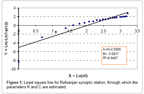
Figure 1: Least square line for Rafsanjan synoptic station, through which the parameters K and C are estimated.
The numerical values of A=K, B and C obtained from Kerman synoptic stations are presented respectively as follows: Kerman: 1.5271, -2.6023 and 5.4963; Kahnooj: 2.4894, -5.3718 and 8.6524; Bam: 1.4619, -2.1969 and 4.494; Baft: 2.3471, -4.6212 and 7.1625; Anar: 1.9472, -3.4531 and 5.8906; Shahrbabak: 2.3925, -4.8376 and 7.553; Sirjan: 2.1545, -3.8827 and 6.0624; Miandeh-jiroft: 1.7545, -2.8968 and 5.2125; Rafsanjan:
Weibull probability function quantities (Pw) are presented in Tables 1-9. These quantities are computed using Weibull scale and Form parameters. Also, vi numerical values, in these Tables (mean of wind speed classes) were computed through equation 1.
With the help of Weibull distribution function, the computation quantities for wind speed occurrence and factual wind speed occurrence over Kerman synoptic station has been drawn in Figures 2-10. Numerical representations of wind speed are distributed in the graphs and are connected by the continuous line drawn with the help of Weibull function. By comparing them, the wind speed disconnected quantities substituted in a curve Contiguous can be observed.
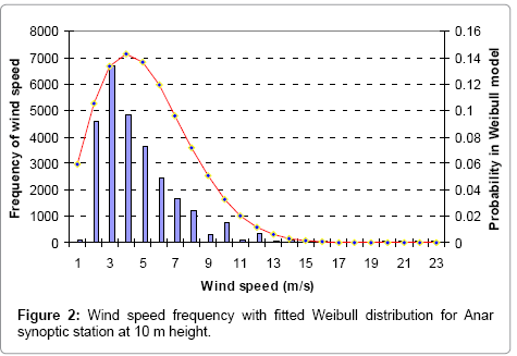
Figure 2: Wind speed frequency with fitted Weibull distribution for Anar synoptic station at 10 m height.
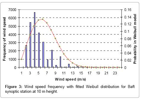
Figure 3: Wind speed frequency with fitted Weibull distribution for Baft synoptic station at 10 m height.
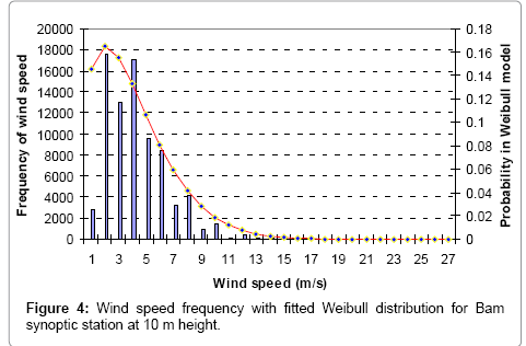
Figure 4: Wind speed frequency with fitted Weibull distribution for Bam synoptic station at 10 m height.
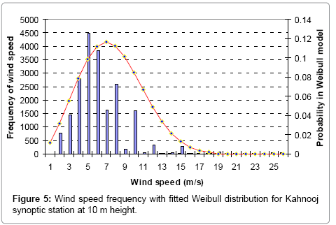
Figure 5: Wind speed frequency with fitted Weibull distribution for Kahnooj synoptic station at 10 m height.
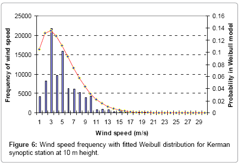
Figure 6: Wind speed frequency with fitted Weibull distribution for Kerman synoptic station at 10 m height.
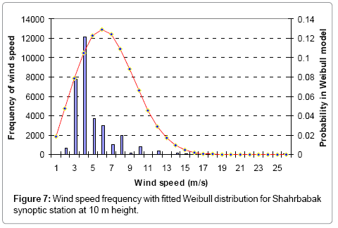
Figure 7: Wind speed frequency with fitted Weibull distribution for Sirjan synoptic station at 10 m height.
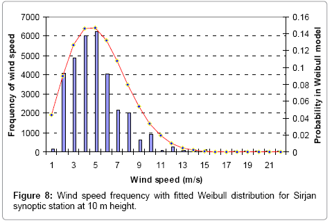
Figure 8: Wind speed frequency with fitted Weibull distribution for Sirjan synoptic station at 10 m height.
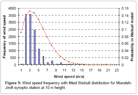
Figure 9: Wind speed frequency with fitted Weibull distribution for Miandeh-Jiroft synoptic station at 10 m height.
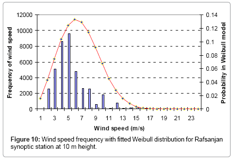
Figure 10: Wind speed frequency with fitted Weibull distribution for Rafsanjan synoptic station at 10 m height.
Calculation of efficacious parameters in wind energy potential estimation
As the scale and shape parameters have been calculated, two meaningful wind speeds for wind energy estimation, i.e. the most probable wind speed and the wind speed carrying maximum energy, can be simply obtained. The most probable wind speed denotes the most frequent wind speed for a given wind probability distribution and is expressed as follows [7]:
 (8)
(8)
The wind speed carrying maximum energy represents the wind speed which carries the maximum amount of wind energy, and is expressed as follows [6]:
 (9)
(9)
The average wind speed (V) and wind speed standard deviation (σ ) can be calculated through the following equations [7]:
 (10)
(10)
 (11)
(11)
where Γ denotes the Gamma function
The probability of wind speeds between  and
and  is given by [8]:
 (12)
(12)
Wind turbines are designed with a cut-in speed, or the wind speed at which it begins to produce power, and a cut-out speed, or the wind speed at which the turbine will be shut down to prevent the drive train from being damaged. For most wind turbines, the range of cut-in wind speed is 3_4.5 m/s, and the cut-out speed can be as highly as 25 m/s [8].
Wind power density
Wind power density The evaluation of wind power density per unit area is of fundamental importance in assessing wind power projects. Wind power density,expressed in Watt per square meter (W/m2), takes into account the frequency distribution of the wind speed and the dependence of wind power on air density and the cube of the wind speed [9]. Therefore, wind power density is generally considered a better indicator of the wind resource than wind speed. Wind power density of a site based on a Weibull probability density function can be expressed as follows [10]:
 (13)
(13)
where ρ is the mean air density (usually taken as equal to 1.225 kg/m3 which depends on altitude, air pressure, and temperature) [11], and Γ denotes the Gamma function. Once wind power density of a site is given, the wind energy density for a desired duration (a month or a year) can be expressed as [12]:
 (14)
(14)
where  is the time period (or duration), for example,
  is 720 hr for monthly duration.
The problem of transforming Weibull parameters at the hub heights of the wind turbines can be easily solved with the compatible features of Weibull distribution. Weibull function facilitates the presentation of the wind speed distribution thereby making it possible for the researcher to transform the wind speed distribution at 10 m height to the distribution at any other height. This is done by applying the so called one seventh power law [13]:
 (15)
(15)
where C2 and C1 are the Weibull scale parameters at heights Z2 and Z1, respectively. Even if the Weibull shape parameter, k, varies with height, the variation is small, and for the present analysis, the shape factor is assumed to be independent of the height.
In the previous studies, in order to obtain total wind hour existence, wind hours in each speed class throughout a year were computed and then the cumulative quantities were achieved [14].
In the present research, a new equation is obtained which provides a simpler and easier method to estimate wind hour existence at an area. The equation is as follows (Mahdi Dehghan):
 (16)
(16)
where WE stands for Wind Existence,  is the unit of measuring the parameter, hour by year, fi is the frequency of wind speed classes or the quantities presented in Table 1, column 4. N is the length of the statistical period under study in a year, and T is the time interval between the wind data records in hours.
The total amount of wind hour existence at the synoptic stations under study was in Kerman 4392.69, Kahnooj 2632.81, Bam 4243.87, Baft 3181.85, Anar 3128.31, Shahrbabak 3852.84, Sirjan 3515.22, Miandeh-Jiroft 1589.74 and Rafsanjan 5950.8 hour by a year
Wind power density is an essential factor in locating places suitable for the installation of wind turbines. At studied synoptic stations, wind power density in Kahnooj, Shahrbabak, Rafsenjan and Baft at heigh of 10 meters from ground level was 439.55, 299.7, 292.68 and 259.48 W/m3 respectively. Meanwhile In the classification of areas suitable for wind turbine installation based on available wind power at 10 meters from ground level, wind power density raging from 200 to 250 W/m3 is considered
As mentioned above, most efficient wind turbines have been designed for a wind speed of 3 meters per second. Meanwhile lowest most probable monthly wind speeds for studied stations at an altitude of 50 meters (the height of the installation of most wind turbines) at all studied stations except Bam, more than 3 meters per second, can be safely observed in Kahnooj, Rafsanjan,Shahre Babak and Baft stations , respectively 8.86, 7.77 and 7.11 m.
According to equation (12), the probability of a wind speed between 3 and 25 m/s in Kahnooj, Rafsenjan, Shahrbabak, and Baft synoptic stations was respectively 96,95,94 and 93 percent of total wind hour existence that in these places has been respectively 2632.81, 5950.8, 3852.84, and 3181.85 hour by year at the height of 50 m. Therefore, the economical operations for wind turbines in mentioned stations are estimated to be about 2527, 5653, 3621 and 2959 hour by year respectively.
The mean wind speeds in all of studied stations is estimated to be more than 6 m/s. Each of these speeds can be the working speed level for wind turbines.
The difference between the most probable wind speed and the wind speed carrying maximum energy in Rafsanjan, Baft, Sirjan, Shahrbabak, Kahnooj, Anar and Miandeh-Jiroft, annually, are less than 5 which show the trivial difference between the maximum probability of wind speed and the wind speed which provides the highest amount of energy in these places.
Finally, the wind power density at 50 meters above ground level, and other mentioned features, Kahnooj, Shahre Babak and Rafsanjan synoptic stations are obtained the potential for the installation of wind turbines and extraction of wind power.