Review Article - (2016) Volume 5, Issue 2
Various aspects of manufacturing and production processes contribute to technological, energetic, and economic efficiency in relevant production. The present paper gives preliminary considerations concerning the influence of biofuel production, and its energetic efficiency on potential fulfillment of agricultural energy demand and consequently sustainability of agricultural production. The energetic efficiency is defined as the ratio of energy obtained from biofuels produced basing on crops from particular area to energy required to satisfy needs of all subsidiary processes assuring correct functioning of plantations on that area.
The effects of energetic efficiency of industrial processes converting agricultural crops onto biofuels also have to be analyzed.
The derived model gives quantitative relations between energy efficiency of sc. “energetic plantations”, energetic efficiency of industrial biofuel processing plants, and energy demand for other types of agricultural production. Investigations are aimed towards determination of the role of biomass as a source of energy, the possibility of assuring energetic self-sufficiency of agriculture and its effect on global energy demand.
An attempt is also made to formulate quantitative basis for describing the idea of sustainable development.
The effects of exclusion of a fraction of crops from food production towards biofuel production are also discussed.
Keywords: Biofuel; Production system; Energetic efficiency; EROEI, Mathematical modelling; Sustainability.
The idea of sustainable development is the main driving force towards the search of roads to stable economic growth accompanied with long-lasting accessibility of natural resources and the values of the natural environment, both indispensable for correct functioning of the single man as well as the whole societies.
The growth of industrial production appears as the cause of natural resources depletion, as well as the reason for degradation of natural environment. It seems, however, impossible to maintain contemporarily achieved standard of life of the present world’s population without supporting further economic growth, based on the development of industry. The growth of standard of life of the human communities as well as development of industrial production is strongly dependent upon availability of energy, which so far is mainly harvested from fossil resources. Two factors are of interest: the first is expected “oil peak”, which can be understood as reaching the maximum of accessible rate of resource logging. As a consequence, after reaching the maximum yield of fossil resource, like petroleum or coal, its availability is expected to decrease. In spite of some controversies concerning estimation of temporal perspective of this peak, its occurrence in some future seems unquestionable. The other factor that has to be taken into account is emission of carbon dioxide inseparably connected to, originated from fossil resources, coal or petroleum derived fuels. An increase of carbon dioxide concentration in atmosphere as well as dissolved in ocean waters brings dangerous consequences to environment, and consequently to human beings. The search of technical solutions which would be able to reduce the negative influence on the environment and to slow down exhaust of natural resources, become important task for contemporary engineers and manufacturers.
At present, it is strongly believed that sustainability can be achieved by means of shifting from fossil resources to renewable ones, which to great extend are bio-resources that come either from “wild” resources or from agriculture.
Agriculture itself is also dependent upon many non-renewable resources, starting from the use of fossil fuels up to use of mineral fertilizers, etc. Consequently, when agricultural production, at least to some extent, has to replace fossil energy resources, it is worth to analyze whether or not, and to what extent this replacement will assure the sustainability of agriculture.
Biofuels, actually not only achieved theoretical, scientific interest, but also reached strong share in fuels’ market. A number of biological resources [1], like seeds, fruits and other parts of various plants, animal fat, etc. are being converted into biofuel, as well as many technologies of this conversion have been elaborated [2-4]. It is supposed, that biofuels become strategically important sustainable energy sources, playing substantial role in mitigation of carbon dioxide emission.
Several papers have been published concerning energetic yield of particular plants, and its effects on sustainability of plantation [5-9]. Several attempts to evaluate quantitative indicators of sustainability have also been published [10]. Estimation of values of some indicators, like EROEI - “Energy return on energy invested” gave input to several conclusions, not necessarily being in agreement. Paper [11] estimates rather good perspectives for biofuels as a factor helping in reduction of CO2 emission as well as showing good potential for meeting future energy demand. The paper gives estimate of actual share of biofuels in global primary energy consumption as equal to 10% and 80% share in total renewable energy production. Similar visions are frequently expressed as point of view by many political officials. On the other hand several researchers [12-14] indicated some problems – namely either too high energy requirements for particular crop production or in global analysis evident lack of arable land that would be sufficient for covering the whole global energy demand, what would introduce strong competition with food production. Consequently, the limits for expansion of biofuel production might be serious.
On the other hand the above mentioned publications indicate importance of biofuels for the worlds and individual Nations’ economies, as well as need for further research to investigate the energetic efficiency of biofuel production systems.
The aim of present paper is an attempt to analyze the effect of biofuel production on sustainability of agriculture by means of recently developed model for energy efficiency of agricultural part of biofuel production [15].
The terms “sustainability” and “sustainable development” are frequently used as synonyms what might lead to some misunderstanding. Namely sustainability might be understood as “plateau” - stagnation - constant state. Sustainable development, in turn, may rather be associated with constant rate of some transition (growth, development). In processes (transitions) occurring in nature constant rate can be expected in situations where space or resources are unlimited. When the available resource is limited, and consequently its amount decreases during transition, the rate of the process varies in time.
In the previous work of Wasiak [16] the use of a kinetic function, usually applied to the description of the physical, chemical or biological processes, was proposed for mathematical modeling of technological or economic processes occurring in conditions of limited resources. The function

where: a, k, n are numerical coefficients, constant in a given process (however, they, as well as x(t) might also depend upon several other parameters). The coefficient, a, represents the full accessible quantity of the substrate undergoing transition e.g. during production, while coefficients k and n characterize the rate of the processing. Variable x(t) describes the quantity (or fraction) converted into the product at an instant of time t. In the case of discrete products, the function describes mass or volume of an assembly of produced item, not the individual item. Coefficients k and n can be used to define so-called half time, t1/2, of the process, which represents the time, in which the degree of the transformation achieves the value a/2, and the rate of the process reaches maximum.
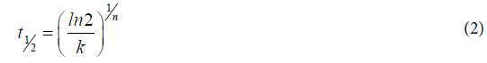
The period of time equal to 2t1/2 one can identify with the life-time of the product on the market. In this time full saturation of the market with the product occurs, and the speed of the production achieves zero. Shape of transformation curves represented by function (1) for various values of coefficients a, k and n, is always sigmoidal, but the level of saturation, and the half times are different. Obviously, the time 2t1/2 is much longer than the life-time of an individual sample of the product.
Similar function of sigmoidal shape assuming the form:
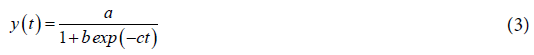
have been used by Bogatov [17] for modeling of mining processes. In this case also coefficients a, b and c define the shape the transformation. Recently, also Manteuffel-Szoege [18] applied such function to the analysis of persistence of pollutant on its environmental and economic effects.
The rate of a process described by function (1) depends on time and is expressed by the following equation:
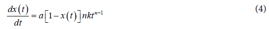
Changes of the processing rate described by equation (4) correspond to typical bell shaped function. The process rate is equal to zero at the beginning, than grows achieving a maximum at,t1/2, and later diminishes reaching zero at the time close to 2t1/2. Basing on equation 4 it is also easy to notice, that the transformation rate is proportional to [1- x(t)], that is in the every instant of the time, t , the transformation rate is proportional to the quantity (or fraction) of remaining not yet processed substrate material. Consequently the saturation of the function described by equation 1, can be interpreted as a result of shortage of raw material.
In the present work the function (1) is a starting point to the analysis of the virtual process for which a fraction of transformed substrate is recirculated back to the supply of substrate. This may be a case when individual item of a product is already worn, and material reclaimed. For the case of biofuel, this concern amount of the fuel that was burned, and CO2 is returned to atmosphere.
Assuming, that only a fraction, α, of the material contained in the final product (e.g. carbon in biofuel) will undergo recirculation, at the instant of time, tz, one can introduce an expression describing the flux of reclaimed material in the form:

Taking into account, mentioned earlier, dependence of transition rate upon the degree of transformed material one can postulate that the flux of recycled material can be simply added to the formula describing the rate of the primary process (equation 4) giving the expression for the rate of a modified process, i.e., the process including recirculation. Therefore the new rate can be expressed as follows:
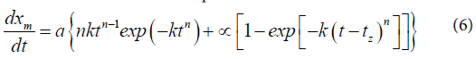
Comparison of functions, dxm(t)/dt, and dx(t)/dt, for arbitrarily chosen values of tz and α is given in Figure 1. It should be noted that the parameter a=1, and tz is presented in the figure as relative value reduced by the half time of the process i.e.:
It is seen that at constant, and relatively low value of parameter α=0,2 the shape of the curve corresponding to the large value of tzrel=1, i.e., for which the recirculation starts at the time corresponding to the half time of the manufacturing process, resembles that for unmodified process for relatively long time, deviating from the later quite late. The observed deviation, however, represents fast increase of the rate. The cases with much shorter time required to start the flux of reclaimed material an increase of rate above the maximum for unmodified process appears approximately at half time of unmodified process, and an increase is even stronger. At longer times all modified courses practically converge.

Figure 1: Transformation rate of modified process as compared to primary one.
| A [km2] | a [km] | Energy yield from plantation area [GJ/ha] | ||||||
|---|---|---|---|---|---|---|---|---|
| 20 | 30 | 40 | 50 | 60 | 70 | 80 | ||
| 1.25 | 0.5 | 15.54 | 23.3 | 31.06 | 38.84 | 46.6 | 54.36 | 62.12 |
| 1.75 | 0.7 | 15.62 | 23.42 | 31.22 | 39.04 | 46.84 | 54.64 | 62.44 |
| 2.25 | 0.9 | 15.64 | 23.46 | 31.28 | 39.1 | 46.92 | 54.74 | 62.56 |
| 2.75 | 1.1 | 15.5 | 23.26 | 31 | 38.76 | 46.5 | 54.26 | 62 |
| 3.25 | 1.3 | 15.52 | 23.28 | 31.04 | 38.78 | 46.54 | 54.3 | 62.06 |
| 3.75 | 1.5 | 15.52 | 23.28 | 31.04 | 38.78 | 46.54 | 54.3 | 62.06 |
Table 1: Values of energetic efficiency, e, for several field areas, and operation width w=0.5 m.
| A [km2] | a [km] | Energy yield from plantation area [GJ/ha] | ||||||
|---|---|---|---|---|---|---|---|---|
| 20 | 30 | 40 | 50 | 60 | 70 | 80 | ||
| 1.25 | 0.5 | 30.42 | 45.64 | 60.84 | 76.06 | 91.26 | 106.48 | 121.68 |
| 1.75 | 0.7 | 31.16 | 46.74 | 62.32 | 77.88 | 93.46 | 109.04 | 124.62 |
| 2.25 | 0.9 | 30.88 | 46.32 | 61.76 | 77.18 | 92.62 | 108.06 | 123.5 |
| 2.75 | 1.1 | 30.66 | 45.98 | 61.32 | 76.64 | 91.96 | 107.28 | 122.62 |
| 3.25 | 1.3 | 30.98 | 46.46 | 61.94 | 77.42 | 92.9 | 108.38 | 123.86 |
| 3.75 | 1.5 | 30.74 | 46.12 | 61.48 | 76.86 | 92.22 | 107.6 | 122.96 |
Table 2: Values of energetic efficiency, e, for several field areas, and operation width w=1.0 m.
| A [km2] | a [km] | Energy yield from plantation area [GJ/ha] | ||||||
|---|---|---|---|---|---|---|---|---|
| 20 | 30 | 40 | 50 | 60 | 70 | 80 | ||
| 1.25 | 0.5 | 58.4 | 87.6 | 116.8 | 146 | 175.2 | 204.4 | 233.6 |
| 1.75 | 0.7 | 62.04 | 93.06 | 124.08 | 155.1 | 186.12 | 217.14 | 248.16 |
| 2.25 | 0.9 | 61.5 | 92.24 | 123 | 153.74 | 184.48 | 215.24 | 245.98 |
| 2.75 | 1.1 | 61.08 | 91.6 | 122.14 | 152.66 | 183.2 | 213.72 | 244.26 |
| 3.25 | 1.3 | 60.7 | 91.06 | 121.4 | 151.74 | 182.1 | 212.44 | 242.8 |
| 3.75 | 1.5 | 60.38 | 90.56 | 120.74 | 150.92 | 181.1 | 211.28 | 241.48 |
Table 3: Values of energetic efficiency, e, for several field areas, and operation width w=2.0 m.
| Number of days for one operation | |||||
|---|---|---|---|---|---|
| A [km2] | w=0.5 m | w=1.0 m | w=1.5 m | w=2.0 m | w=2.5 m |
| 1.25 | 45 | 25 | 15 | 15 | 10 |
| 1.75 | 60 | 30 | 20 | 15 | 15 |
| 2.25 | 75 | 40 | 25 | 20 | 15 |
| 2.75 | 95 | 50 | 35 | 25 | 20 |
| 3.25 | 110 | 55 | 40 | 30 | 25 |
| 3.75 | 125 | 65 | 45 | 35 | 25 |
Table 4: Number of days *) needed to perform one agricultural operation, as a function of plantation size, and operation width, d, of the equipment, *) shadowed unrealistic values.
Basing on equation (6) one can derive a formula describing the progress of a modified process. This obviously can be written as:
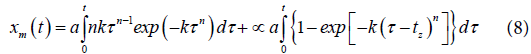
where τ have the meaning of current time, and resulting dependence x(t) is a function of upper limit of the integral. The equation (8) shows that resulting process is a sum of two fluxes of a substrate, the first one correspond to the virgin material, while the second to reclaimed one. The contribution of each one is determined by the factor, α.
Numerical integration
Numerical integration of the equation (8) was performed in order to visualize changes in the course of the process caused by returning some fraction of reclaimed material to the process. The computations were carried out by means of the trapezoid integration algorithm enabling presentation of the results as a function of upper limit of integration. Results are shown in Figures 2 and 3.
Data presented in Figure 2 illustrate the effect of starting time tz on the course of investigated process. When tz is relatively long i.e., the late start of recirculation, than the course of the process during early part of the process development resembles the unmodified course, apparently reaching the same level of saturation, from which rather late it deviates to larger degrees of conversion. The curves corresponding to shorter tz, deviate much earlier without exhibiting any trend of leveling off. It can be concluded that even relatively small fraction of recirculated substrate material is able to affect substantially the course of transition process. The sooner starts reclaiming, the stronger effects are observed (Figure 2).
The data presented in Figure 3 show, in turn, the results of starting time variation in the case when fraction, α, of the reclaimed material is much higher, and equal to 0.4. It is clearly seen that character of the transformation curves is very similar to that shown in Figure 3. Only observed deviations from unmodified process are much more pronounced – the curves at the same instant of time reach much higher value of the conversion. Similar trend is also observed with respect to the location of the starting time of recirculation. The shorter, tz, is the more pronounced effect is achieved. Comparison of both figures suggests that an increase of fraction, α, of the reclaimed material causes rather quantitative effects on transformation, while, tz, exhibits rather qualitative influence on the shape of conversion curves. An increase of each of those parameters causes extension of the process to higher available degrees of conversion, what can be interpreted as causing higher level of sustainability of the process (Figure 3).
The figures shown above consider rather limiting values of parameters. What one could expect in reality is also an increase of a fraction of recirculated substrate, α, during the time of the process. In spite that such calculation have not been carried out, comparison of both figures lead to the conclusion that for each value of tz,the plot of the transition progress with time under condition of time dependent, α(t), would be located between a pair of curves corresponding to the same, tz, presented in both figures above.
In the case of biofuel production, and its influence on agriculture’s sustainability, the recirculated substrate is the carbon dioxide emitted to the atmosphere during burning of the biofuel. The results show that, even relatively low fraction is returned, the effect on the continuation of the transition is clearly visible, while an increase of returned fraction causes very pronounces effect. The other factor is the instant of time when recirculation occurs. This is dependent upon two factors: first is the moment at which the fuel is burned, while the second is connected to the rate of growth of plants. This later factor is much dependent upon type of the plant: for the case of some plants e.g. cereals - it is part of the year, in the case of a tree it is several years before it can be converted onto biofuel. Some contribution to this time is also given by the time required for transportation and conversion of biomass onto biofuel. Some effect, resulting of diffusion time of carbon dioxide in atmosphere could also be considered, it seems however, that plants as well as places of burning fuel are relatively uniformly distributed, and consequently diffusion effects can be neglected. The effects of time shift shown on Figures 2 and 3 show that in each case an increase of conversion above saturation is clearly observed, and substantial hindrance is not observed.

Figure 2: Progress of the processes conducted at the same, low value of a=0,1 and several values of time of beginning of material return tz .

Figure 3: Progress of the processes conducted at the same, higher value of a=0,4 and several values of time of beginning of material return tz.
Consequently, the above results suggest that production, and use of biofuel does not negatively affect sustainability of agricultural production, at least in the part concerning agricultural use of biofuel. It is a result of recirculation of carbon dioxide from biofuel back to plants.
Taking into account critical remarks [19,20] made towards determination of EROEI index used in the literature, the new model of energetic efficiency of biofuel production in agricultural production system was introduced in [15]. The model expresses energetic effectiveness, ε , related to one year of production of agricultural subsystem, as follows:
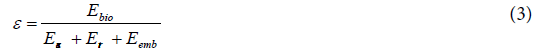
where: EbioM. – is energy obtained from the field, Eex – is energy expended on tillage operations, Etr – is energy consumed for transportation outside of fields, Eemb – is a fraction of embodied energy contained in production means, that is spend during tillage operations and transport executed during production year.
The contributing energies are further expressed as follows:
Energy obtained from the plantation equals to:
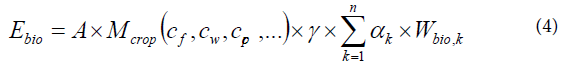
where: A – is plantation area,  – is crop yield dependent upon concentrations: cf – fertilizer,
cw – water, ccp – crop protection means, maintained during cultivation. γ – general mass fraction of biofuel in the crop, αk – mass fraction of k species of biofuel, Wbio,k – low caloric value of k-species of biofuel.
The other term is the energy consumed on the field during agrotechnical operations:
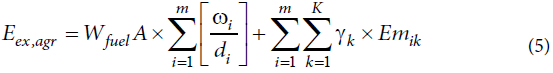
where: ωi – the fuel consumption per unit of the distance passed during the individual agro-technical process, di – the width of the land strip operated in the single course of i-th operation,
Wfuel – the low caloric value of the fuel used for operations (might be fossil fuel or biofuel),
m – the number of the agro-technical operations (in each one of the operations the width of the worked field, di , and the consumption of fuel, ωi , can be different), γk – is a fraction of embodied energy contained in one of the, k technical means employed at i-th operation (machines, fertilizers, etc.). It may be estimated e.g. as ratio of the time of particular operation to the total expected life time of particular equipment, Emk– is embodied energy contained in k-th technical mean.
The last term concerns transportation of goods (including crops) outside of the field. This term is especially important for big plantations that have to be arranged in several fields separated sometimes by quite long distances. Contribution of transport is also significant when crops have to be transported through long distance to industrial facilities for processing. It is expressed as:
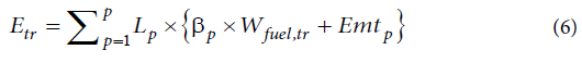
where: Lp – is a distance driven outside of the field in p- th route, βp – is fuel consumption during p route, Wfuel, tr – is low caloric value of the fuel used in transport, Emtp – is fraction of embodied energy of a given transportation mean corresponding to the unit of distance driven.
As seen from the above formulas individual contributions to the energetic efficiency are dependent upon various factors. Especially, Ebio, and Eex, agr depend i.a. on plantation area, A, while Etr does not. Also embodied energy terms Emik, and Emtr do not depend explicitly on A, in spite that some contribution to it (e.g. energy embodied in crop protection means or fertilizers) might depend upon plantation area. It means that efficiency, ε , depend upon the size of plantation in a complicated manner, affected by various relationships. Numerical computations were performed to get deeper insight into relations described in the model.
It is worth to mention that the value, Ebio, in the numerator of formula is the value obtained at the end of production system (including industrial one) i.e., it correspond to the energy contained in the ready biofuel obtained from agricultural system being under consideration. Such approach gives the value characterizing efficiency of agricultural subsystem in a relative way. It, however, gives a possibility to estimate similar characteristic, εtot, of a bigger system built of several subsystems, connected in series e.g. agricultural and industrial subsystems, using a simple, easy to derive, formula:

where ε1, ε2 are the values of efficiency determined for subsystems.
This formula is also valid for subsequent agro-technical operations performed in the same production field.
Numerical computations
Numerical computations, using equations given above, were aimed towards establishing dependencies of energetic efficiency upon technical parameters of agricultural operations. Results presented here are extension of the results given in [21]. Since consideration of relatively large plantations was assumed, the computations additionally included calculation of time needed for any operation, and under assumption of maximum daily working time – the number of days needed to perform operation on particular field were evaluated. Moreover, it was assumed, that after reaching this maximum time the equipment is transferred back to the base. This obviously increases the distance driven back and forth outside of the field. Schematic view of assumed plantation’s topological structure is given in Figure 4.

Figure 4: Schematic view of assumed topological structure of plantation.
Analysis of the situation shows that after starting the work equipment is moved from the base driving the distance, c, and drives back and forth on the field till the maximum working time is reached. At this moment returns to the closest to the base field border being on the distance from the base equal to sum of c+a1/J. The fraction of the distance, a1, is determined by the number of days, J, needed for elaboration of the whole field. The distance, which have to be driven next day before the operation on field can be started is, c+a1/J. Return to the base after the second day work requires the distance c+a1/J., Similarly, each next day of work is associated with analogous increase of distances driven outside of the field. Some subsequent day this daily driven distance is increased by contribution of the distance, l1, between first and second fields, and so on. Finally the sum of all contributions for the fields can be expressed as:
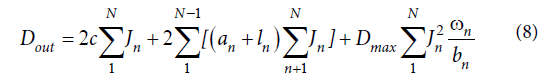
where, ωn, denotes the width of operation strip on the field, n, and, N , denotes total number of fields.
Computations were performed assuming plantation structure composed of five fields of equal sizes with dimensions b=0,5km, and a – variable, separated by the distance, l=0,2 km, and he distance from the base equal to c=5km. Values of the width of operation strip, ω, were assumed, namely equal to 0.5m, 1m, 1.5m, 2m, and 2.5m.
Low caloric value of the fuel used for running machines was taken as: 36MJ/dm3, and for biofuel 34.6 MJ/dm3. Fuel consumption by agricultural machines was assumed 0.3 dm3/km. Machine speed was estimated as 6 km/h , since maximum daily allowable working time was assumed 10 h, the resulting daily working distance driven on the field was equal to 60 km.
Result show that for all cases distance driven on the field was substantially bigger than that, driven outside. It is also clear, that machine with wider operational strip assures shorter both distances. Also both distance are increase with an increase of plantation area.
Tables given below show dependence of energy effectiveness, ε, as a function of plantation area, and the width of operation strip. The values of, ε, are computed for several values of energy yield from the unit of plantation area (in GJ/ha). The values taken into account correspond to the approximate energy yields obtainable for various “energetic” plants (about 30 GJ/ha can be obtained from rapeseed plantation, a little bit smaller value one obtains from wheat plantation for bioethanol production, while about 80 GJ/ha may be achieved in bioethanol produced from sugar beet). Values of energy efficiency presented in tables below are computed for five agricultural operations performed on the fields, under assumption of equal energy consumption for each operation. Subsequent tables show values of energetic efficiency for different operational width of the machines used (Tables 1-3).
It can be easily recognized that the values, presented in the tables, rather slightly depend on plantation area, but are strongly dependent upon the width of operation strip – consequently the appropriate choice of the equipment is playing substantial role. Obviously, they also strongly depend upon energy yield from area unit of plantation, i.e. the kind of plants being cultivated. Each kind of plant requires, however, different procedures for converting it onto biofuel. The factors neglected in present analysis are: energy embodied in production means (machines, tools, crop protection substances, fertilizers, etc.) It seems that this contribution is not very high, but it needs further studies.
Values of energetic efficiency, presented in tables above, vary between 15 and 250 depending on type of plants cultivated, distance between fields, and size of plantation (the later contributions are rather small). Further reduction of energetic efficiency should be expected to occur in industrial part of production system where the conversion of biomass to biofuel occurs, and due to energy needed for transport of biomass to industrial facility, that might be quite energy consuming because possibly large distances, and large amounts of biomass that undergoes transportation. As indicated in [22] estimations based on life cycle analysis show that biodiesel production from palm oil requires two – three times more energy than cultivation of plants and oil extraction, while in the case of bioethanol, produced from cassava fruits, the energy needed for conversion is even four times higher than energy demand for agricultural processes. This means that energy efficiency would be reduce 20% to 50% in industrial conversion operations. This is obviously valid for specific plants, and specific climatic conditions, so those proportions may vary depending on localization of plantation, and also upon technology of conversion. Consequently, one can expect efficiency of biofuel production system being between 5 and about 100, depending mainly on type of plant cultivated, amount of energy spend during agricultural operations and energy consumption during industrial conversion onto biofuel. Important for achieving high energetic efficiency is therefore appropriate choice of agricultural and industrial, and technology optimization of logistics inside as well as outside of plantation.
The problem appropriate choice of equipment is not only associated with a decrease of energetic efficiency, but also with time required to perform agricultural operations. Table 4 gives an example illustrating a variety of cases (Table 4).
It can be recognized that at several choices of operation width, ω, individual agricultural operation take too long time. Each operation in production systems requires some “time window”, which in agriculture is determined mainly by climatic and biological requirements. Operations which last too long are simply not acceptable. In such cases more efficient machinery is needed.
Two models presented in present paper indicate that recirculation of carbon dioxide, although after some delay contributes to sustainable development of agriculture. As to the question whether or nor agriculture can be self-sufficient with respect to energy needed for production, it can be concluded that in fortunate case of good choice of plants, tillage, and subsequently conversion technologies, one unit of area of arable land dedicated to “energetic” plantation may be sufficent for providing energy to more than hundred such units of other plantations. In the worse cases this would be only 5 units of area that could be cultivated on the basis of energy obtained from one unit of “energetic” plantation. This clearly indicate meaning of good choice of the type of plantation as well as choice of technologies needed for cultivation and conversion onlto biofuel.
“Energetic” plantations can be localized on pieces of land separated from lands being already cultivated, as well as from waste lands. The later case is obviously better solution with respect of food production from arable lands, but might be worse from viewpoint of conservation of wild land. Another aspect that might make the situation even better is use of agricultural waste rather than useful crops e.g. use the straw rather than grain of corn to convert it onto biofuel. This approach requires, however, development of appropriate conversion technology that would assure good energetic efficiency of conversion processes. Some Authors suggest to use non-edible fruits from various plant e.g. castor oil. In such a case, one has to consider that although edible fruits are not “wasted” for industrial conversion, but arable land – is wasted.
Energetic efficiency of agricultural subsystem depends upon:
a) The technical parameters of applied machines,
b) The distance traveled on the field during agricultural operations, which is mostly contributing into energy consumption
c) The number of operations (and consequently upon production technology),
d) The distances travelled between fields (which depends on the degree of dispersion of the plantation and upon the sizes of individual fields – The vary big fields force an increase of movement of machinery outside of the field, it however appear to have weaker influence than the distances driven on the fields.
e) The distance between the plantation and the processing installation - transportation of the grain. This transport showing not so big absolute values of energy consumption, does not substantially affect the total energetic effectiveness of the production system. The energy consumption depends on transportation means characteristic – mainly the ratio of volume capacity to fuel consumption per unit of the distance.
Energetic efficiency depends on the scale of the industrial production subsystem, which extorts the suitable scale (size) of the plantation, and also decides about the consumption of fuels (energy) during the agro-technical operations and transportation.
The estimated values of energetic efficiency are mostly dependent upon energy yield from particular plant being cultivated. The most pronounced technical factor is the efficiency of agricultural machines, since the distance driven on the field is the most contributing to energy consumption
Production organization might also affect energetic efficiency, especially by correct choice of inter plantation and outside of plantation logistic solutions.
The research have been performed under financial support from Bialystok University of Technology. Statutory Research Project WZ/S/1/2015 financed from scientific grant from Ministry of Science and Higher Education (MNiSW).
1The paper corresponds to the “Honorable Speaker” lecture presented at the conference, Plant Genomics 2016” Brisbane, Australia