Journal of Climatology & Weather Forecasting

The periodicity of some biosphere phenomena, as climatic cycles [1-3], mass extinctions [4], abrupt changes of biodiversity rate [5,6] and others [7-9] in the course of geological time have been noted by many researchers. The question is, what determines such periodicity, and whether these events, differing by nature, are somehow connected among them. These questions are a subject of debate. The objective of this publication is to show that the above phenomena have a common cause relating to global carbon cycle. This conclusion may be done by means of a newly suggested global redox carbon cycle model [10]. This model has some features that distinguish it from the others.

Redox carbon cycle model is based on the two known geologic concept - plate tectonics and organic cycles. Plate tectonic concept [11-13] asserts that plates, covering the Earth surface, move permanently making a motion reminiscent of the movement of the escalator. In the zone of mid-Atlantic ridge magma erupts onto the surface and, coming into the contact with ocean water, hardens to form a new plate. In the other place of the Earth (in Wadati - Benioff zone) the plates, moving towards each other, collide. One of them, bending and moving down under the other, is absorbed by magma.

To these views I added assertion that in zone of plate collisions (subduction zone) with participation of continental plates under higher temperatures thermochemical sulfate reduction occurs. Sedimentary organic matter, one of the reaction substrates, interacting with gypsum from oceanic water, is oxidized and produces CO₂, which lifting onto the Earth surface, fills “atmosphere - hydrosphere” system and exerting an impact on photosynthesis development. The lithospheric plates’ movement indirectly influencing on photosynthesis is the first specific feature of the suggested redox carbon cycle model.

The orogenic cycle concept [7] asserts that the intensity of the vibrations of the Earth’s crust over the geologic history was unequal. There were relatively short periods, named by orogenic periods, and the subsequent relatively extended periods of quiet development of the crust, named by geosynclynal periods. The geosynclynal and the orogenic periods both make the orogenic cycles which Rutten [7] has named the Earth’s pulse.

Organic periods are characterized by intensive mountain building and active volcanism, accompanying with eruptions and entry of the large masses of igneous rocks onto the Earth’s surface. Geosynclynal periods are characterized as the time of quiet Earth's crust development, of slow plate movement, as the time of reduction of volcanic activity and mountain building. It is the time for intensive weathering processes, accumulation of precipitation and increased photosynthesis.

I have supposed that organic periods correspond to the time of quick lithospheric plates’ movement and massive entry of CO₂ onto the Earth surface what stimulates photosynthesis development. Geosynclynal periods correspond to the time of dominant role of photosynthesis what leads to the depletion of CO₂ in the “atmosphere - hydrosphere” system. The link of the plates’ movement with the organic cycles is the second specific feature of the redox carbon cycle model. Besides, differing from the orogenic cycles concept, I consider that CO₂, derived in oxidation of sedimentary organic matter in subduction zone, but not juvenile CO₂, is the main contributor to the “atmosphere - hydrosphere” system.

The third feature, differing the redox carbon cycle model from the others [14-16], is the assertion that carbon turnover as not a simple transition of the element between geospheres and biosphere, but a conversion of carbon from the oxidized state, presented by CO₂, bicarbonate and carbonate ions in the “atmosphere – hydrosphere” system, into the reduced state, presented by different biogenic forms, produced in photosynthesis and in the following transformations. The reverse transition is realized via respiration of living organisms, via microbial and chemical oxidation accompanying transformations of “living” matter after the burial. Among the oxidative processes the final oxidation of organic matter in subduction zone is dominant.

The suggested sequence of geological events assumes the CO₂ injections into “atmosphere – hydrosphere” system and the achievement of maximal concentration of CO₂ occur in organic period. In geosynclynal period it implies depletion of the pool of inorganic carbon at the expense of photosynthetic CO₂ consumption. Thus, the global redox carbon cycle formally can be presented as a closed loop consisting of the two branches – oxidative and reductive. It has two remarkable points, one of which is photosynthesis, where the oxidized carbon species turn into the reduced state; another point provides the reverse transition (Figure 1).

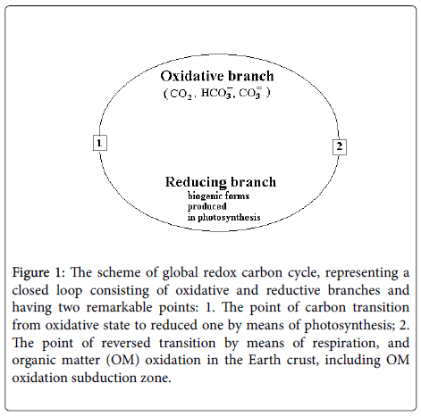
Figure 1: The scheme of global redox carbon cycle, representing a closed loop consisting of oxidative and reductive branches and having two remarkable points: 1. The point of carbon transition from oxidative state to reduced one by means of photosynthesis; 2. The point of reversed transition by means of respiration, and organic matter (OM) oxidation in the Earth crust, including OM oxidation subduction zone.

The participation of the two key natural global reactions in the cycle: photosynthesis (1) and sulfate reduction (2)

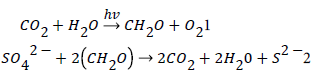
Provides an excellent opportunity to check the validity of the model’s conclusions due to participation of the different natural form of carbonates, sedimentary organic matter, marine sulfates and sulfides that can be examined and compared with the products of the assumed reactions. The studies of isotopic variations of the elements in the above natural objects play a special role in checking the validity of the model, since they are described by the known physico-chemical laws.

Below we’ll describe the assumed mechanism of functioning of the redox cycle of carbon and then give some examples of the use of chemical and isotopic characteristics to substantiate it.

In a short-term orogenic period of the cycle carbon dioxide, produced in thermochemical sulfate reduction, fills the “atmosphere – hydrosphere” system, which involves the common chemical exchange system “carbon dioxide – bicarbonate – carbonate”:

The system, as it stemmed from the isotopic data [17], is close to equilibrium. In the following long-term geosynclynal period due to photosynthesis the concentration of CO₂ in the system decreases. Carbon dioxide concentration from the maximal meaning, achieved in the orogenic period, reaches its minimal meaning by the end of the geosynclynal period (Figure 2).

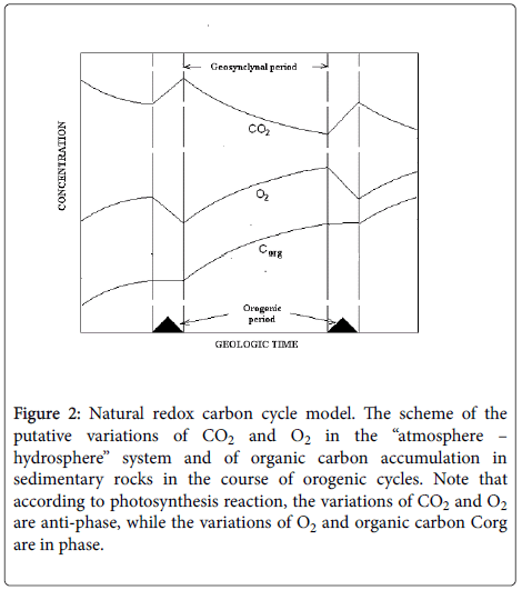
Figure 2: Natural redox carbon cycle model. The scheme of the putative variations of CO₂ and O₂ in the “atmosphere – hydrosphere” system and of organic carbon accumulation in sedimentary rocks in the course of orogenic cycles. Note that according to photosynthesis reaction, the variations of CO₂ and O₂ are anti-phase, while the variations of O₂ and organic carbon Corg are in phase.

Another product of sulfate reduction, hydrogen sulfide, coming onto the Earth surface, in parallel with CO₂, interacts with atmospheric oxygen and turns back into oxidized form completing redox cycle of sulfur. Thus carbon and sulfur cycles are coupled. The sulfate reduction is the coupling point and an essential element of carbon turnover periodically providing CO₂ into the “atmosphere – hydrosphere” system. Arguments, confirming the interaction of carbon and sulfur cycles, are given in [10]. Atmospheric oxygen demonstrates quite different behavior. In orogenic period O₂ concentration drops, since it is used for oxidation of H2S and the reduced igneous rocks, lifting onto the Earth surface simultaneously with volcanic gases. In geosynclynal period, when photosynthesis becomes dominant, oxygen demonstrates antiphase character relative to CO₂ changes, since the latter is a substrate, whereas O₂ is a product of the global photosynthesis reaction (Figure 2).

Taking into account, that the residence time of carbon, as sedimentary organic matter, is much more than the life time of the “living” matter, organic matter can be regarded as the product of photosynthesis instead of “living mater”. Its behavior can be easily deduced from the analysis of the reaction (1).

In orogenic period burial rate of organic matter remains at the level which was achieved by the end of the previous cycle, since it was assumed that the rate slightly depends on tectonic activity. In geosynclynal period, when photosynthesis becomes dominant, the burial rate of organic matter occurs in proportion to oxygen. The accumulation of organic matter in sediments is in parallel with oxygen growth in the atmosphere. Their variations are in phase. Some facts, confirming the existence of orogenic cycles and expected behavior of the above parameters are given in [10]. Isotopic data provide additional arguments.

According to the model, after filling “atmosphere - hydrosphere” system with CO₂ in orogenic period a gradual depletion of inorganic carbon pool takes place due to photosynthetic CO₂ consumption in the subsequent geosynclynal period. The depletion is accompanied by carbon isotope fractionation and results in 13C accumulation in residual carbon dioxide due to isotope effect, known as Raliegh effect [18]. Note, that other species of inorganic carbon, due to equilibrium between them, change their isotopic composition by the same manner. The newly produced organic matter, according to the Raleigh law, also experiences the similar isotopic variations.

Let’s analyze natural carbon isotopic data, obtained by Derry et al. in 1992 [19] (Figure 3). The authors summarized the available from the literature data on marine carbonates from Neoproterozoic (ca. 900-540 Ma) in three widely separated basins and claimed the observed isotopic shifts as post-depositional alteration. They paid attention to high positive values of δ13C of marine carbonates (+4 ÷ +8%) during most of the studied period and explained them as a result of low burial rate of organic carbon. The sharp negative isotope excursion they attributed to the Varangian (ca. 600 Ma) and Sturtian (ca. 780 Ma) glacial episodes.

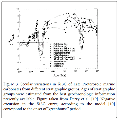
Figure 3: Secular variations in δ13C of Late Proterozoic marine carbonates from different stratigraphic groups. Ages of stratigraphic groups were estimated from the best geochronologic information presently available. Figure taken from Derry et al. [19]. Negative excursion in the δ13C curve, according to the model [10] correspond to the onset of “greenhouse” period.

Quite different interpretation of the results may be done on the basis of the global redox carbon cycle model. According to the model, the observed isotopic shifts of carbonates are the result of photosynthesis, but not post-depositional effects. The anomalous 13C enrichment of Neoproterozoic marine carbonates, as compared with those in the subsequent periods [20,21], is a manifestation of the Raleigh effect, resulted from high extent of pool depletion of inorganic carbon due to greater duration of Neoproterozoic orogenic cycles (greater extent of pool depletion) as compared with Phanerozoic ones.

The negative isotopic shifts of carbonates (Figure 3) evidence that both peaks have appeared in orogenic (warming) periods. The negative sign of isotopic shifts is provided by oxidation of sedimentary organic matter which is known to be enriched in 12C. A significant influx of “light” CO₂ (enriched in 12C) from subduction zone in the orogenic period makes the carbon of inorganic pool to be "lighter". On contrary, the 13C accumulation in carbonates, observed close to the Sturtian (ca. 780 Ma) and Varangian (ca. 600 Ma) glacial episodes, is explained by Raleigh effect, resulting in the 13C enrichment of CO₂ achieved by the end of the corresponding geosynclynal periods.

Another example of isotopic data application is based on the use of the differences between carbon isotope composition of coeval carbonates and sedimentary organic matter, deposited in the same facial conditions. Following to actualism principle, carbonates can be considered as analog of the carbon dioxide in the past atmosphere, whereas coeval sedimentary organic matter may be considered as analog of the “living” matter. Hence, the difference between carbon isotope composition of coeval carbonates and organic matter maybe regarded as analog of 13C isotope discrimination in photosynthesis in the past. It was designated as ε parameter [2].

Here some comments are required. As known, photosynthesis consists of two reciprocal processes of CO₂ assimilation and photorespiration [22]. CO₂ assimilation is responsible for growth of biomass, photorespiration for its decline. The total effect is determined by the contribution of each of them and depends on the CO₂/O₂ concentration ratio in the environment. Both processes are in reciprocal relations, i.e., the strengthening one of them is accompanied by a weakening of the other [23]. From the recent photosynthesis studies it was found [24,25], that each process is accompanied by carbon isotope fractionation with effect of opposite sign.

Bearing this in mind, it may be concluded that CO₂ assimilation results in 12C enrichment, whereas photorespiration is followed by 12C depletion of biomass [26]. Hence, high CO₂/O₂ ratio in the environment provides the 12C enrichment, whereas low CO₂/O₂ ratio leads to the 12C depletion of biomass.

In accordance with the above, the periodic changes of CO₂/O₂ ratio within the orogenic cycle from the maximal meaning in the orogenic period to the minimal meaning by the end of geosynclynal period causes the gradual 13C enrichment of biomass and a decrease of isotopic parameter ε (Figure 4). This can be used to distinguish orogenic cycles.

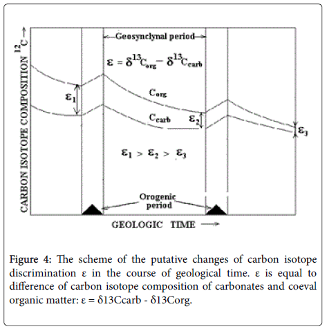
Figure 4: The scheme of the putative changes of carbon isotope discrimination ε in the course of geological time. ε is equal to difference of carbon isotope composition of carbonates and coeval organic matter: ε = δ13Ccarb - δ13Corg.

Taking into account that with every new orogenic cycle, an average oxygen concentration in the atmosphere increases, causing intensification of photorespiration, one should conclude that “living” matter and hence the buried organic matter should be enriched in 13C with each subsequent cycle. This assertion is supported by direct measurements of carbon isotope composition of organic matter and its derivatives (petroleum), observed in the course of geological age [2,27,28]. Confirming the validity of the model, it is possible to proceed to the consideration of the nature of the periodicity of some biosphere phenomena.

Climatic cycles from the standpoint of global redox carbon cycle model

According to the model, each organic cycle begins with the growth of CO₂ concentration in the organic period and is completed with its drop at the close of the geosynclynal period. The role of CO₂ as the main component of a “greenhouse” gases is a well-known fact [29]. The periodic filling/depletion of the “atmosphere – hydrosphere” system with CO₂ within the organic cycle on the background of the cycles repeatability provides alternating warming - cooling. There is direct relation between CO₂ concentrations and Earth’s temperature that was even used for determination of paleotemperatures [3].

In this approximation the organic cycles coincides with climatic ones. It was shown, that due to the increase of the average oxygen concentration in the atmosphere, isotopic ε parameter, characterizing the end of each subsequent cycle is lesser than corresponding ε value of the previous one. It means that should be coherence between climatic cycles and ε values. Indeed, Popp and co-workers [30] disclosed such a coherence between the ε values for samples of sedimentary organic matter in Cenozoic and corresponding climatic cycles found by Fischer [1] independently. Hayes et al. [2] having examined carbon isotope composition for over than 5000 samples of coeval carbonates and sedimentary organic matter spanning Precambrian and Phanerozoic, found statistically significant difference of ε values in interglacial periods and those in period of glaciations. These results were supported by Huang et al. [31] and by Bornemann et al. [32].

The periodic abrupt changes in biodiversity rate correlate with orogenic cycles

A periodicity in biodiversity rate (a rate of appearance of the new fauna and flora species per geological unit) in time was marked by Liebermann and Melott [33]. Igamberdiev and Lea [34] found that maximum of biodiversity rate corresponded to the maximum in O₂ concentration in the atmosphere. The assumption was confirmed by close coherence of the curves illustrating time dependence of biodiversity rate and other parameters, strongly related to oxygen concentrations. The peaks of all curves fully coincide and correspond to oxygen maximum [34].

According to the redox model, the periodicity in biodiversity rate is caused by the periodic increase of oxygen concentration in the Phanerozoic atmosphere which takes place at the end of geosynclynal period of each cycle.

The physical sense of this link is quite clear. The elevated O₂ concentrations in the atmosphere stimulate (photo) respiration in photosynthesizing organisms, which is followed by superoxide radicals formation. The radicals attack gene molecules causing mutations. Though in a cell there are some enzymes, which destroy radicals reducing them to H₂O and O₂, at the time of oxygen growth the enzymes fail to cope with the abundance of radicals and to diminish their amount to the safe level. As a result, mutations appear and biodiversity rate increases properly. It is notable, that the end of geosynclynal period is characterized, besides a high oxygen concentration, with the lowest temperatures often ending with glaciations. Thus the glaciations may be used as an indirect indicator of the increased biodiversity rate.

A good example in nature, reflecting the link between biodiversity rate and the glaciations, is the Great Ordovician Biodiversification Event, the most rapid and sustained increase in marine Phanerozoic biodiversity. It agrees with the transition from greenhouse period of early Ordovician to the sudden Mid Ordovician icehouse period that lasted till Late Ordovician [35].

The converse assertion is also true. The growth of CO₂ concentration in the marine system in post-Cambrian time (Late Devonian, end-Permian and end-Triassic), that caused “greenhouse” effect and oxygen depletion of water, was followed by the biodiversity loss in marine taxa [36,37].

As shown before, ε parameter is a function of CO₂/O₂ ratio. It gets the lowest value at the end of geosynclynal period. It means there should be coherence between ε parameter and biodiversity rate. This correlation was found by Rothman [38] for land plant families and marine animals.

Repeatability of mass extinctions and orogenic cycles

Mass extinctions have occurred repeatedly in the geological past [39,40]. Unlike to high biodiversity rate, associated with high O₂ concentration achieved by the end of geosynclynal period, mass extinctions of organisms are connected with the transition from geosynclynal period of one cycle to the orogenic period of the next. The transition is characterized by dramatic loss in O₂ concentration in the “atmosphere - hydrosphere” system. The abrupt drop in O₂ atmospheric level is the most likely cause for mass extinctions of aerobic organisms.

The conditions, under which mass extinction used to occur, are characterized by a set of traits: anoxic environment, global warming, negative carbon isotope excursion and sea level rise [41]. This is the very set, that characterize the onset of orogenic period of each cycle [10]. It draws to the conclusion that mass extinction is associated with adverse changes in the environmental conditions. Among the set of traits a lack of oxygen is the most critical. The authors of [37] have shown that the organisms less adapted to the reduced oxygen content die first. They are representatives of the upper links of trophic chain, mainly belonging to aerobic organisms. The most primitive photosynthesizing organisms, anaerobes and facultative aerobes, much better adapt to low oxygen conditions and have more chances to survive. Moreover, they propagate and are capable to produce oxygen, gradually restoring aerobic conditions. By the end of the geosynclynal period high oxygen environment stimulates recreation of the trophic chains, but on a new qualitative level.

Mass extinction of organisms is considered to be the main source of organic matter for the formation of sedimentary rocks rich in organic matter (black shale, domanicoids, etc). Most likely organic matter is associated with a plankton community, inside which there is a circulation from a high-diversity eukaryote to high-biomass bacterial colonies [37].

The changes in the global redox carbon cycle after achieving ecological compensation point. The manifestation of biosphere events before and after achievement ecological compensation point

Since photosynthesis is a key element of the global redox carbon cycle, its evolution made the cycle to evolve too. The main stream of the photosynthesis evolution was the oxygen accumulation coupled with CO₂ concentration decrease in the system. Indeed, at the moment of photosynthesis origin, oxygen was present in the atmosphere in negligible amount [7]. Since then O₂ concentration gradually, but steadily has grown until it reached a stationary level close to the present day. Another product of photosynthesis, sedimentary organic matter, has accumulated in the Earth crust in proportion to O₂ in the atmosphere. At once after the origin of photosynthesis the appearance of oxygen was detrimental to photosynthesizing organisms. To survive, organisms were forced to adapt, having invented photorespiration. The latter has become an essential part of their metabolism. It is likely, at the same time the mechanism of photosynthesis regulation has appeared in the form of oscillatory coupling of CO₂ assimilation/ photorespiration [42].

The first primitive photosynthesizing organisms, termed as C3- organisms, apparently had the ability to adjust the assimilation/ photorespiration ratio, depending on the ratio of CO₂/O₂ in the environment. It is known [22] that photosynthesizing organisms of C3- type have so-called compensation point, at which there is a balance between CO₂ assimilation and photorespiration. It means that the amount of assimilated carbon becomes equal to the amount of oxidized carbon. The compensation point determines physical limits of plant survival. If to place a set of plants into a closed chamber at different, but constant CO₂ levels [43], after a while in all cases the concentrations of CO₂ and O₂ in chamber atmosphere are stabilized, reflecting different ratio of CO₂/O₂. Tolbert et al. [44] assumed that the same feedback mechanism operates in nature, and results in stabilization of CO₂ and O₂ in the atmosphere.

In connection with the global carbon cycle system, the concept of the compensation point should include, besides the respiration processes in plant community and in the “living” matter, all the oxidation processes of sedimentary organic matter in the Earth’s crust, including those proceeding in subduction zones in sulfate reduction [10]. Then the state, termed as ecological compensation point, will correspond to the state when all the reduced carbon, produced in photosynthesis will be equal to the carbon, returned back from the reduced state into inorganic species (CO₂ - HCO₃- - CO^3- ₂).

When reaching an ecological compensation point, the system becomes extremely sensitive to the collisions of separate lithospheric plates and long-term orogenic cycles are completely replaced by shortterm oscillations, called climatic oscillations. Climatic oscillations have appeared prior to ecological compensation point. Orogenic cycles closer to the point has been become shorter and aftermath they have fully disappeared.

It is difficult to define certainly the time of achieving the ecological compensation point, but most likely it has appeared after Miocene. In fact, in Miocene it was marked the growth of atmospheric oxygen [45,46] and the increase of biodiversity [47,48] indicating the orogenic cycle. However, frequent changes of warming and cooling, having observed in Miocene, has indicated on the proximity of the system to the ecological compensation point. The cooling period was ultimately culminated with glaciations. Some other traits clearly showed that in Miocene there was a transition from the geosynclynal period of one cycle to the orogenic period of the next. Indeed, in the middle of Miocene (14,8 to 14,5 Ma) there were considerable tectonic events, followed by intense volcanism and magmatism [49,50]. It agrees with sea level rise, with the observed distribution of thermophylic vertebrates and with mass extinction of some other species [39,51,52].

In addition, this agreed with the appearance in Miocene of the last notable wave of oil generation [53,54] that indicated that the rocks, rich in organic matter, were formed in Miocene. The mass extinction, mentioned before, has provided organic matter for these rocks. All the traits allowed concluding that in Miocene there was the last orogenic cycle.

Taking into consideration all the above, it is possible to answer the question, how the biosphere events have manifested themselves both in terms of orogenic cycles and in terms of climatic oscillations. As it follows the model [10], orogenic cycles and climatic oscillations have the same physical nature associated with the collisions of the moving lithospheric plates that affected on photosynthesis and the related sequence of events in biosphere.

In both cases the vibrations are characterized by alternating phases of warming and cooling, each of them is associated with drastic change in CO₂ and O₂ concentrations in “atmosphere – hydrosphere” system, or, by another words, with high and low CO₂/O₂ concentration ratio, accordingly with aerobic and anaerobic (low oxygen) environment. The transition from the cooling to warming phase is associated with dramatic changes in the species of terrestrial and marine community as well. It is often followed by mass extinction, by sea level rise, by isotopic shifts in carbonate and organic matter carbon, in carbonate oxygen, by isotopic shifts in sulfate and sulfidic sulfur, in nitrate nitrogen and by isotopic shifts of some other trace elements (Sr, Fe, Mo, Cr, etc) [55]. It should be stressed that in most cases the different traits appear synchronously relating to the transition.

Nevertheless, there are some specific features related to different duration of orogenic cycles and climatic oscillations. Long-term orogenic cycles exert global effect over the whole planet, while shortterm climatic oscillations are limited to the region, where they arise. By studying of biosphere events in terms of orogenic cycles it is necessary to average their characteristics over large period. Therefore the processes separated by small time intervals are considered as synchronous. On contrary, in case of climatic oscillations, even the events, separated by insignificant time intervals, can be distinguished from each other.

For example, in conditions of orogenic cycles by studying secular isotopic variations of carbonate carbon and of sulfate sulfur from sea water [55,56] they may be considered as synchronous. It allows concluding that carbon and sulfur cycles are coupled and that the sulfate reduction is the coupling point. Another case is presented in the work of Owens et al. [57]. By studying one of the climatic oscillations in the Cretaceous (Oceanic Anoxic Event 2, spanning the Cenomanian-Turonian boundary) the authors found the interval of peak magnitude for carbon isotopes precedes that for sulfur isotopes with an estimated offset of a few hundred thousand years. It allows concluding that carbon isotope effect is associated with photosynthesis, while sulfur isotope effect appeared later in the sulfate reduction reaction [10].

According to the suggested model of carbon turnover, moving lithospheric plates generate orogenic cycles consisting of two periods. In a relatively short-term orogenic period, when lithospheric plates move quickly, due to frequent plates’ collisions considerable amounts of CO₂, produced in sulfate reduction in the subduction zone, enter the “atmosphere – hydrosphere” system. The source of CO₂ is sedimentary organic matter of continental plates subjected to oxidation. Carbon dioxide which fills the “atmosphere - hydrosphere” system in the orogenic period, stimulates photosynthesis. In a longterm quiet geosynclynal period, when plates move slowly and collisions are rare, photosynthesis becomes dominant. Due to photosynthetic consumption, CO₂ concentration in “atmosphere - hydrosphere” system drops. Thus the irregular lithospheric plates’ movement provides periodic CO₂ injections that determine uneven photosynthesis development.

The uneven photosynthesis development leads to the periodicity of many processes in the biosphere related to photosynthesis, such as climatic cycles, changes in the rate of biodiversity, the repeatability of mass extinction on land and in ocean, the repeatability of the formation of deposits rich in organic matter.

The evolution of photosynthesis led the carbon cycle to the ecological compensation point, i.e., to the state when all the reduced carbon, produced in photosynthesis becomes equal to the carbon that returns back from the reduced state into inorganic species. After achieving this point long-term orogenic cycles were replaced with short-term climatic oscillations.

The manifestations of biosphere events in terms of orogenic cycles and in terms of climatic oscillations are the same because of the equal nature of their origin. It is supported by the same set of traits characterizing them.

The difference is in that in terms of orogenic cycles, characteristics of events averaged over long interval allows establishing global correlations in time. In terms of climatic oscillations, due to short-term periodicity of the oscillations, the detail study of their characteristics allows examining the sequence of the processes related to the oscillations.