Research Article - (2018) Volume 6, Issue 3
Numerical prediction of fog evolution remains difficult due to its complex processes that require adequate representation of the local perturbations in weather models despite the progress made in advance weather prediction models. The performance and sensitivity of the Weather Research and Forecasting (WRF) model in reproducing fog episodes over Akwa Ibom international airport (AKIA) Nigeria for the first time in West Africa was studied. Some real cases of radiation fog over AKIA were simulated using a set of parameterization schemes to simulate warm fog and visibility limits. Seven fog events were selected for model validation and sensitivity studies in this research work. The use of Kunkel (1984) empirical relationship result showed good agreement between simulated horizontal visibility limits using Liquid Water Content (LWC) when compared with observation. The modeled diurnal patterns of temperature, relative humidity and wind speed were also evaluated with the observed. It was found out that the model also captures the diurnal pattern and the value with very slight biases. These slight biases however, do not affect model results except where overestimation of wind speed and temperature could give rise to an earlier dissipation of fog. Fog estimation through temperature and relative humidity profile is as a result of the turbulent mixing within fog that causes the homogenization of the layers where the fog is present. The result showed evolution of fog through quasi-saturated state between temperature and relative humidity defining fog characteristic onset pronounced by surface inversion.
Keywords: Fog occurrence; Onset; Dissipation; Evaluation; Slight bias; Reproduce
Fog is defined as “suspension of very small, usually microscopic water droplets in the air, generally reducing horizontal visibility near the earth´s surface to less than 1km according to the World Meteorological Organization [1]. Fog is a boundary layer phenomenon that typically develops near the surface of a stable nocturnal atmospheric boundary layer. Its development is strongly influenced by surface conditions, the effects of the underlying surface on fog can be direct when the surface is influenced by vertical profiles of wind, temperature, humidity, and other local forcing through horizontal heterogeneities, or indirect through modification of radiative properties of the atmosphere by microphysical processes and varying aerosol spectra. As described by Cotton et al., fog is not treated as a separate cloud genus; instead it is defined in terms of its microstructure, horizontal visibility, and proximity to the earth’s surface [2]. The study focuses on radiation type of fog which is the commonest.
Prediction of fog have evolved over few decades of studies where numerical models of different levels of complexities in terms of computational requirements, data inputs and model microphysics have been deployed in resolving this mesoscale phenomenon to produce forecast with explicit spatial and temporal details. Fog detection with good spatial and temporal resolutions is therefore, of great interest to applications in traffic safety and other human endeavors. Usually, a fog episode has a large impact on maritime, land transportation and most particularly in aviation safety. Visibility degradation due to fog formation endangers traffic safety, as such methods of forecasting/ nowcasting of fog need improvement by using various modeling techniques including state-of-the-art numerical models. Modeling has given us the tool to better understand the atmosphere and its processes. This in turn has led to a reliable meteorological forecasting. Previous studies based on non-hydrostatic simulations have shown the advantages of high-resolution model in capturing the detailed evolution and structure of atmospheric systems phenomena. However, the advantages of high-resolution model seem to be highly cased and are geographically dependent [3]. Contrary to coarse resolution simulations, the high-resolution model allows convective activities to be resolved in an explicit manner. Numerical models for weather predictions have been incorporated using a variety of physical schemes taking into account different characteristics of specific locations of the world [4]. It cannot be an understatement that forecasting the areal extent of radiation fog is very important to aviation and highway travelers. Studies have validated the direct correspondence between dense fog and significant societal and economic impacts. However, the indirect effects of fog are undeniable. Fog indirectly impacts the environment in two main ways: by reducing visibility; and by serving as a liquid aerosol which can maintain contact with structures and vegetation for several hours. Unfortunately, no national statistics data on the impact of radiation fog is available in Nigeria for fog-related air crashes and road accidents were archived (to the best knowledge of the authors). Reduced visibility associated with fog can have other adverse effects in various areas in Nigeria. The presence of fog has been linked to piracy and armed robbery against ships and aircraft in the Niger Delta [5]. It is a logical extension of these studies to say that, the presence or absence of fog in a battlefield would certainly impact on military operations [6].
This work investigated the performance of a state-of-the-earth weather model using a good combination of parameterization schemes for simulating radiation fog as suggested [7] to simulate and predict warm fog events using Weather Research and Forecasting (WRF) modelling tool applied at Jaipur, India. His set of schemes was chosen because of the similarities in weather phenomena between India (Asia) and Nigeria (West Africa). Subsequently, validation of the model sensitivity to the already observed radiation fog was addressed by comparing model output with observational data and the use of [8] empirical relationship between liquid water content and horizontal visibility in radiation fog event. Further sensitivity studies was also performed to possibly determine spatial and temporal distribution of radiation fog, its onset, duration, vertical extent and horizontal visibility limits. Details of model configuration are highlighted in Table 1.
| General Setting | |
| Time | 2012-12-01_00:00:00 – 2013-02-28_18:00:00 |
| Grid Size | Domain 1: 39500 x 39500 Domain 2: 13000 x 13000 |
| Horizontal resolution | Domain 1: 12000 x 12000 Domain 2: 4000 x 4000 |
| Vertical resolution | 38 levels |
| Parameterization Scheme | |
| Land surface | Unified NOAH Land surface |
| Urban Canopy model | Single layer |
| Boundary layer | Quasi-Normal Scale Elimination (QNSE) |
| Microphysics | Lin et al. 1983 |
| Longwave radiation Shortwave radiation |
Rapid Radiative Transfer Model (RRTM) Dudhia, (1989) |
| Convection scheme | Grell-freitas |
| Cumulus scheme | Kain-Fritch (New Eta) |
| Urban Parameters determined by Land Use | |
| Anthropogenic heat flux | |
Table 1: ARW numerical setup for model reference run.
Geographical location and climate of the study area (Akwa Ibom)
Akwa Ibom State lies between latitude 4° 32″N and 5° 53″ N and longitudes 7° 25″E and 8° 25″E, it covers a total land area of 8,412 km2, encompassing the Qua Iboe River Basin, the western part of the lower Cross River Basin and the Eastern part of the Imo River Basin. With an ocean front which spans a distance of 129 kilometers from Ikot Abasi in the west to Oron in the east [9]. The climate of Akwa Ibom State can be described as a tropical rainy type with mean annual rainfall of 3000 mm to 4000 mm, depending on the area, characterized by two seasons, namely, the wet or rainy season and the dry season. In the south and central parts of the State, the wet or rainy season lasts for about eight months but towards the far north, it is slightly less. The rainy season begins about March-April and lasts until mid-November. Akwa Ibom State is always at the constant influence of the southwesterly monsoon winds throughout the year. The mean maximum annual humidity of 96% and above is recorded at nighttime and early hours in the morning while between 60% and 68% recorded during the afternoon. Thick cloud cumulonimbus type is commonly experienced in the months of March to November. Evaporation is high with annual values ranging from 2000 mm to 2500 mm [10].
Two episodes of radiation fog that occurred over Uyo from 13th - 15th and 22nd - 25th December 2012 were selected. Parameters such as relative humidity, temperature, horizontal visibility, wind speed and direction over Akwa Ibom International Airport (AKIA) were obtained from the archive of Nigerian Meteorological Agency (NiMet) and compared with those of the WRF model outputs (Figure 1). These parameters were compared with respect to fog onset, development, and dissipation. Subsequently, Liquid Water Content (LWC) from the model output is applied in order to test WRF sensitivity to fog onset, thickness, and duration. Boundary and initialization data for the simulation was sourced from the archive of Global Forecast System (GFS) at the National Centre for Environmental Prediction (NCEP) Final (FNL) data. The data has the temporal resolution of 6 hour and a spatial resolution of 1o by 1o grid applied on a nested domain with a horizontal resolution of 12 km and 4 km and 38 vertical levels.

Figure 1: Map of Akwa Ibom State showing the location of Akwa Ibom International airport.
The model simulation produced liquid water content as one of the direct output variables. While this variable denotes the amount of cloud water in the air, it does not directly represent the presence of fog. Therefore, when comparing cloud liquid water content (LWC) to visibility, formulations are needed to convert LWC to visibility limitations to determine fog. Kunkel (1984) discussed this conversion through an extinction coefficient β, defined as:
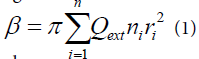
where:
Qext is the normalized extinction cross-section; and
ni is the number density for cloud droplets of radius ri.
Since cloud microphysics parameterization information is not always available in forecast models, Kunkel (1984) further provided an empirical relationship between the liquid water content (LWC) and the extinction coefficient (β):
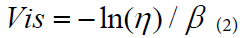
where LWC is in gm-3. This β can then be translated into visibility by:
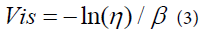
where η is the threshold of contrast normally taken as 0.02.
From these empirical relationships, it can be evaluated that when LWC > 0.02 gm-3, visibility is less than 1 km, thus it can be classified as fog. Since the air density is close to 1 kgm-3, the threshold of fog occurrence when LWC is 0.02 gm-3 is equivalent to liquid water content at 0.02 gkg-1, which was used as the threshold for fog identification in this research work.
Model validation of simulated fog events
The first period of the two episodes consists of three days between 13th and15th while the second period consists of four days between 22nd and 25th. METAR report at AKIA indicates that these periods (13th to 15th and 22nd to 25th) of fog events were characterized by favorable synoptic conditions (not shown) for the development of radiation fog, i.e. high-pressure systems with low-pressure gradient and clear skies, calm winds allowing the nocturnal radiative cooling required to saturate the air [11,12]. The sensitivity of the WRF model in simulating the occurrence of radiation fog via the model output variable LWC was performed by selecting seven fog events. The result in Figure 2(a) indicates that, for spatial and temporal distributions of liquid water content simulated by WRF model, there are corresponding variations in horizontal visibility distributions and these variations appear only when the amount of liquid water content is above the threshold value (> 0.02 gm-3). The result (circled plots) shows that when LWC ≥ 0.18 gm-3, horizontal visibility reduces to about 100 meters and below, for threshold values between 0.14 ≤ LWC ≤ 0.18 visibility was between 200 - 400 meters, also where 0.1 ≤ LWC ≤ 0.14 horizontal visibility improved to about 500 meters. The circled plots on both panels show reasonable consistency in the spatial distribution of the same variable of LWC to temporal horizontal visibility evolution of the already observed warm fog onset, its development and dissipation. The result indicates that colors brighter than dark blue (right panel) for the simulated temporal distribution of LWC were equivalent to horizontal visibility less than 1km (left panel), or otherwise fog. Although these figures, as stated above does not clearly represent the evolution of radiation fog properties as expected, it has, however, presented an empirical temporal confirmation of the model sensitivity to the simulated variable, and in this case liquid water content suggesting a high level of confidence in the model results and in the empirical relationship between LWC and horizontal visibility in simulating fog occurrence [13].

Figure 2: Spatial and temporal distribution of simulated horizontal visibility (left panel) LWC (right panel) at 0300, 0600 and 0900 UTC of (a) 13th; (b) 14th; and (c) 15th December, 2012.
Based on meteorological observations of radiation fog episodes, the evolution and spatial distribution of atmospheric variables such as visibility, specific humidity, wind speed, synoptic patterns, and the vertical variation of temperature stratification were analyzed during these fog episodes. Figure 3 shows time series plots of model outputs and observations for (a) relative humidity (%); (b) wind speed (m/s); and (c) air temperature (°C), these are parameters considered as key variables in fog evolution in this research. The present-day mesoscale models have flaws in representing relative humidity [7] since most relative humidity variations occurring in the boundary layer are caused by changes in temperature (cold) biases in numerical models. Surprisingly, the result in Figure 3 (a) shows that the WRF model reproduces the minimum and maximum epoch in relative humidity very well and in agreement with the observed. The observed highest humidity was around 98% on 13th December at 0600 UTC, this was well reproduced by the model as 100% at the same time. The model and observation have a same diurnal pattern with obvious little biases between 1200 and 1500 UTC. The wind speed was also well reproduced by the model having the same diurnal pattern but with overestimation between 0900 and 1200 UTC. The model overestimates wind speed when turbulent mixing increases at sunrise which doesn’t have much effect on the present study that focuses on the occurrence and severity of fog before sunrise. The highest value of 5.0 ms-1 was recorded by the model at 0900 UTC as compared to 3.0 m/s observed [14]. The air temperature was well reproduced having a same diurnal pattern and almost no biases. Figure 3(c) shows a good prediction skill for temperature by the WRF model as it successfully reproduces the minimum and maximum epoch for temperature very well when compared with the observed. The maximum temperature reaches around 31.1°C on 13th December at 1200 UTC and which is well captured by the model (32.0°C). The minimum temperature was observed to be 22.5°C on 13th December 2012 at 0600 UTC, also the model reproduces it as 23.0°C. It can, therefore, be suggested that on the overall, the model satisfactorily simulated diurnal temperature, relative humidity, and wind speed.

Figure 3: Diurnal patterns of simulated and observed (a) relative humidity; (b) wind speed; and (c) air temperature from 0600 UTC of 13th to 2100 UTC of 15th, December, 2012 over AKIA.
To further evaluate the sensitivity of WRF model in simulating the onset, duration and time of dissipation of fog occurrence over the study area, the WRF output from 22nd - 25th December 2012 was again used. Figures 4(a) and (b) show spatial distributions of modeled visibility for 22nd and 23rd respectively from 0400 UTC to 0900 UTC while (c) shows the observed time series of visibility from 0300 UTC, 22nd to 0800 UTC 23rd. Fog was observed to occur for four hours as morning radiation fog from 0300 to 0800 UTC and the model also show the occurrence of fog over the study area and its surrounding form 0300 to 0800 UTC (though 0300 UTC is not shown here it did occur as fog’s widespread at 0400 UTC already confirms this) and visibility started increasing from 0700 UTC in both observed and modeled plots and finally disappears at 0900 UTC. In the second day, 23rd (Figure 4 (b)), radiation fog was also observed between 0300 to 0800 UTC (METAR form supports this fog schedule). However, the visibility was observed as 400 m while the WRF model result (Figure 4 (c)) slightly overestimated it as 500 m at 0600 UTC, the model simulated thick fog at the onset but with a slightly patchy behavior during its dissipation. The fog lifted shortly after sunrise as a result of solar radiative heating, which increases the temperature at the surface. The third period corresponds to the 24th December 2012, (Figure 5 (a)) with a total of five hours of observed warm fog. It is a clear case of pure radiation fog developed during the early hours and dissipated at sunrise. The fog was established at 0300 UTC and dissipated at 0800 UTC with a possible progressive transformation into low clouds because of the decrease in relative humidity at 10 meters at 0800 UTC. The visibility time series (Figure 5 (c)) shows that at 0400 UTC horizontal visibility slightly increased, this is seen from the spatial distribution of liquid water content (Figure 2(a)) at the same time and this slight increase is assumed to be characteristics of deep radiation fog. The fourth period corresponds to the 25th December 2012, (Figure 5 (b)) with a total of 5 hours of thick fog. Figure 5 (c) showed that the fog was established at 0100 UTC and dissipated at 0700 UTC, with a possible progressive transformation into low clouds, however, the fog on this day was not as thick as the preceding day simulated by ARW model as visibility was estimated to be about 200 m at 0600 UTC. It is therefore shown that WRF was able to capture the onset, duration, and dissipation of fog occurrence and its associated poor visibility.

Figure 4: Hourly modeled spatial visibility (km) from 0400 UTC to 0900 UTC for (a) 22nd, (b) 23rd while (c) time series of visibility (km) at AKAI from 0300 UTC, 22nd to 0800 UTC, 23rd.

Figure 5: Same as Figure 4 but from 24th - 25th December, 2012.
Fog estimation through temperature and relative humidity profile
Turbulent mixing causes the convergence of temperatures at different heights to approximately the same value. Thus, many studies evaluate fog thickness through the vertical profile of temperature. However, because of the non-availability of temperature measurements at different vertical heights at AKIA, this study adopted the method used by Teixeira and Pedro [15]. Figure 6 shows the vertical evolution of temperature and relative humidity profiles. The profiles result seems to be related as expected during fog episode, since close to the surface, there exists a quasi-saturated state between temperature and relative humidity. A pronounced surface inversion can be seen on the temperature profile, defining a characteristic of onset of fog at 0300 UTC, this characteristic trend is reflected clearly on the relative humidity profile at the same time. By 0600 UTC, from the surface, a well-mixed layer continued to form in both temperature and relative humidity. If this is compared with the results shown in Figure 6, it is possible to identify this mixed layer as the fog itself. The mixed layer is a characteristic of deep radiation fog [16,17]. At 0900 UTC the inversion is now located at the fog’s top, where a strong radiative cooling process is active, as such, temperature profile becomes slightly unstable due to the solar heating of the surface and the consequent generation of more turbulence leading to fog dissipation. In general, the simulated structures of both temperature and relative humidity are quite realistic when compared with the observations [18-21].

Figure 6: Simulated vertical profiles of temperature (a, c & e) and relative humidity (b, d & f) at 0300, 0600 and 0900 UTC for 23rd December, 2012.
Thus, the overall objective of this work was to study some real cases of radiation fog events over AKIA and to identify the relevant and essential physical processes that cause warm fog formation and dissipation. The sensitivity of Weather Research and Forecasting (WRF) model, by using its Advanced Research core (ARW) was evaluated through the use of Kunkel (1984) empirical formulations on model output variables. The validation study showed that the fog’s onset, growth and its dissipation for seven episodes were reasonably well simulated. The model estimated minimum values of visibility in agreement with observations for four episodes, while slight overestimation and underestimation occurred. A model sensitivity study was further conducted through the use of the vertical profile of some boundary layer variables which shows a very good agreement in their diurnal patterns. Fog onset was determined using vertical profiles of temperature and relative humidity while the duration and spatial distribution of fog were obtained from the empirical distribution of liquid water content. The fog dissipation stage was again reasonably well simulated by the model. The model further shows the dynamical processes as shown by the inversion layer in the temperature and relative humidity profiles close to the surface as the driving factor responsible for the formation of radiation fog.
The methodology followed in this study is rather simple and cannot account for all the features and processes in simulating the formation and dissipation of fog. While numerical models are available, they are still much more difficult to use for operational boundary layer predictions due to both computational and data initialization reasons, leaving some space for the practical use of simpler models such as one-dimensional (1D). However, more detailed verification of spatial patterns for many cases are needed, the use of satellite imagery will be a valuable source of information for this purpose, especially over West Africa where the temporal and spatial distribution of validation data is coarse and unavailable for modelers. The temporal resolution of observed data over the study area has affected the sensitivity of our ARW model result as a comparison was limited to specific periods during observed fog episode. It is hereby recommended that more detailed validation of the model based on high temporal resolution is required where the model’s sensitivity to other parameterization schemes, cumulus schemes and different microphysical and physical processes can be evaluated over West Africa to accurately present the best scheme and physical process best for fog simulation and forecast.
The second author appreciated the financial support of the Nigerian Meteorological Agency (NIMET) for sponsoring her through the course of her Master’s program in the Federal University of Technology, Akure. The observed data of the study area was collected from NIMET data archiving center. We also appreciate the anonymous reviewers for their suggestions towards the improvement of this manuscript.